How Computers Understand Images: A Beginner's Tour of Computer Vision and AI

We live in a world saturated with images. Each day, we process countless visual stimuli—faces of loved ones, text on screens, clouds drifting across skies, and cars navigating busy streets. For humans, this visual processing happens so naturally that we rarely pause to consider the magnificent complexity behind it. Our brains interpret depth, recognize patterns, and extract meaning from light in ways that feel effortless.

But how do machines "see"? How do we teach computers to make sense of the visual world?

This question lies at the fascinating intersection of neuroscience, mathematics, and artificial intelligence. When a computer processes an image, it's not "seeing" in any human sense—it's analyzing numerical data, detecting patterns, and applying algorithms. Yet through this fundamentally different approach, we've created systems that can diagnose diseases from medical scans, drive vehicles, and recognize faces in photographs.

Let's embark on a journey through the landscape of computer vision and AI—exploring how machines interpret the visual world, the core techniques that make this possible, and what this means for our shared future.

The Digital Canvas: How Computers Represent Images

When you look at an image, you perceive a continuous scene with countless details. But to a computer, an image is a grid of discrete values—a matrix of numbers. This fundamental difference shapes everything that follows in computer vision.

"To a human, a picture is worth a thousand words. To a computer, a picture is worth a million numbers."

Pixels: The Atomic Units of Digital Images

Every digital image consists of pixels (short for "picture elements")—tiny squares of color that, when arranged in a grid, create the images we see on our screens. Each pixel stores specific values:

• In a grayscale image, each pixel represents brightness with a single number (typically from 0 to 255, where 0 is black and 255 is white)
• In a color image, each pixel typically contains three values representing the intensity of red, green, and blue channels (RGB)

Let's see how this works in practice with a simple Python example:

import numpy as np
import matplotlib.pyplot as plt
from skimage import data

# Load and crop grayscale image
coins = data.coins()
coins_cropped = coins[90:140, 90:140]  # 50×50 crop

# Define 8×8 patch
x, y = 14, 16
patch = coins_cropped[x:x+8, y:y+8]

# Plot composite
fig, axs = plt.subplots(1, 3, figsize=(18, 5))

# Image with highlighted patch
axs[0].imshow(coins_cropped, cmap='gray', vmin=0, vmax=255)
axs[0].set_title('Cropped Grayscale Image')
axs[0].add_patch(plt.Rectangle((y, x), 8, 8, edgecolor='lime', facecolor='none', lw=3))
axs[0].axis('off')

# Zoomed-in patch (scaled correctly)
axs[1].imshow(patch, cmap='gray', interpolation='nearest', vmin=0, vmax=255)
axs[1].set_title('Zoomed-In Patch (8×8)')
axs[1].axis('off')

# Numeric matrix of pixel values
table = axs[2].table(cellText=patch, loc='center', cellLoc='center')
axs[2].axis('off')
axs[2].set_title('Pixel Values (Brightness)')

plt.tight_layout()
plt.savefig("coins_representation.png", dpi=300)
plt.close()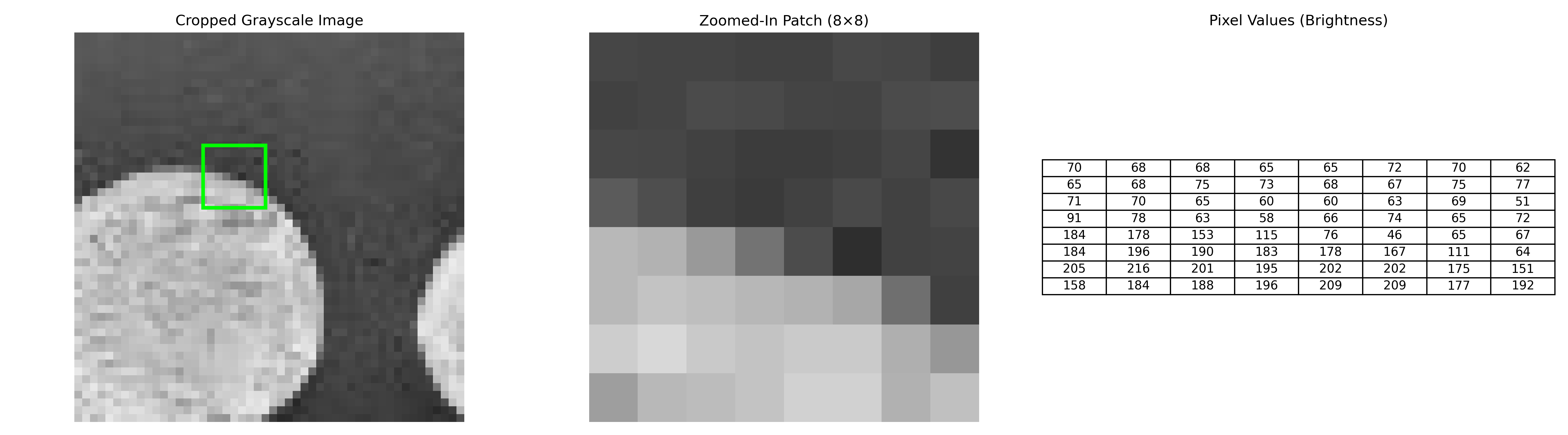

This code loads a sample image of coins from scikit-image and displays it alongside a small section of its numerical representation. What you see as a clear image of coins, the computer sees as a matrix of numbers, each representing the brightness at that position. The higher numbers (closer to 255) correspond to lighter areas, while lower numbers represent darker regions.

The RGB Color Model

Most digital images use the RGB color model, where each pixel contains three channels: Red, Green, and Blue. By mixing these primary colors at different intensities, we can represent millions of colors.

Below is a simple 5×5 synthetic example. We randomly generate three small matrices—one for each color channel—and stack them into a color image. We also isolate each channel visually and show their corresponding numeric values.

import numpy as np
import matplotlib.pyplot as plt

# Step 1: Create random 5×5 matrices for each channel
np.random.seed(42)  # For reproducibility
R = np.random.randint(0, 256, (5, 5), dtype=np.uint8)
G = np.random.randint(0, 256, (5, 5), dtype=np.uint8)
B = np.random.randint(0, 256, (5, 5), dtype=np.uint8)

# Step 2: Stack into RGB image
RGB = np.stack([R, G, B], axis=-1)  # Shape: (5, 5, 3)

# Step 3: Create figure
fig, axs = plt.subplots(1, 4, figsize=(16, 4))

# RGB Image (enlarged using nearest-neighbor interpolation)
axs[0].imshow(RGB, interpolation='nearest')
axs[0].set_title("RGB Composite")
axs[0].axis('off')

# Channel matrices
for i, (matrix, title) in enumerate(zip([R, G, B], ['Red Channel', 'Green Channel', 'Blue Channel'])):
    ax = axs[i + 1]
    ax.table(cellText=matrix, loc='center', cellLoc='center')
    ax.set_title(title)
    ax.axis('off')

plt.tight_layout()
plt.savefig("random_rgb_5x5.png", dpi=300)
plt.show()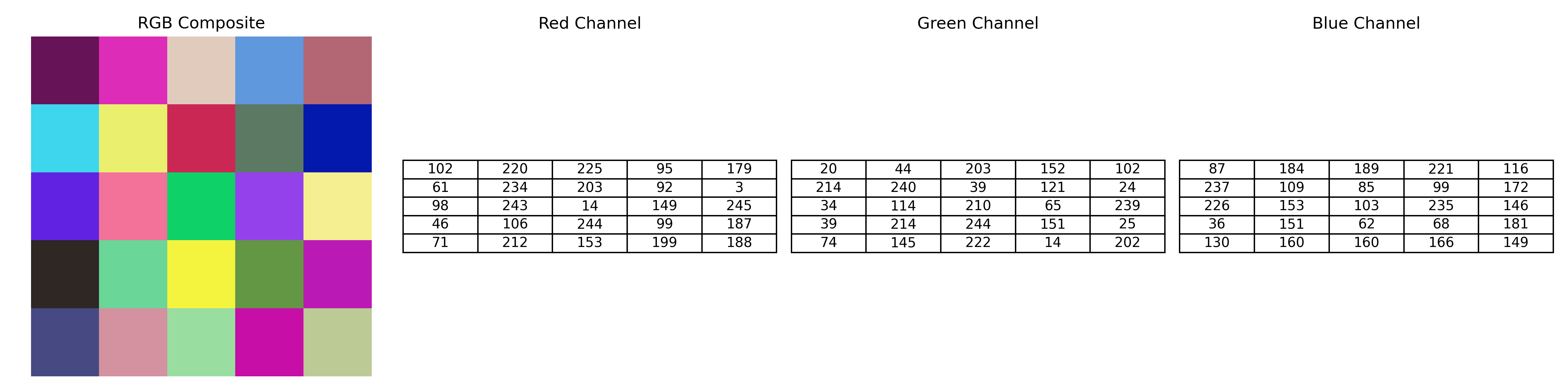

This example demonstrates how a color image is composed of three separate channels. When we isolate each channel, we can see how they combine to create the full-color image.

Note: In the matrix labeled "RGB (Averaged)", the values are not the sum of R + G + B. Instead, each value is the average of the corresponding red, green, and blue intensities:

[ \text{RGB}_{\text{avg}}[i,j] = \frac{R[i,j] + G[i,j] + B[i,j]}{3} ]

This averaging gives us a grayscale representation of the pixel's overall brightness, staying within the 0–255 display range.

The shape of the RGB array reveals its three-dimensional nature:

• Height × Width × Channels → 5 × 5 × 3 in this case.

From Pixels to Features: Teaching Computers to See

While pixels provide the raw material for computer vision, they're just the beginning. Much like how humans don't perceive individual photoreceptor signals but rather assembled features like edges, shapes, and textures, computers must transform raw pixel data into meaningful features.

Edge Detection: Finding Boundaries

One of the most fundamental operations in computer vision is edge detection—identifying the boundaries between different objects or regions in an image. Edges typically occur where there's a significant change in pixel intensity.

from skimage import feature, filters
import numpy as np

# Load a sample image
camera = data.camera()

# Apply different edge detection methods
edges_sobel = filters.sobel(camera)
edges_canny = feature.canny(camera, sigma=2)

# Display the results
fig, axes = plt.subplots(1, 3, figsize=(15, 5))

axes[0].imshow(camera, cmap='gray')
axes[0].set_title('Original Image')
axes[0].axis('off')

axes[1].imshow(edges_sobel, cmap='gray')
axes[1].set_title('Sobel Edge Detection')
axes[1].axis('off')

axes[2].imshow(edges_canny, cmap='gray')
axes[2].set_title('Canny Edge Detection')
axes[2].axis('off')

plt.tight_layout()
plt.show()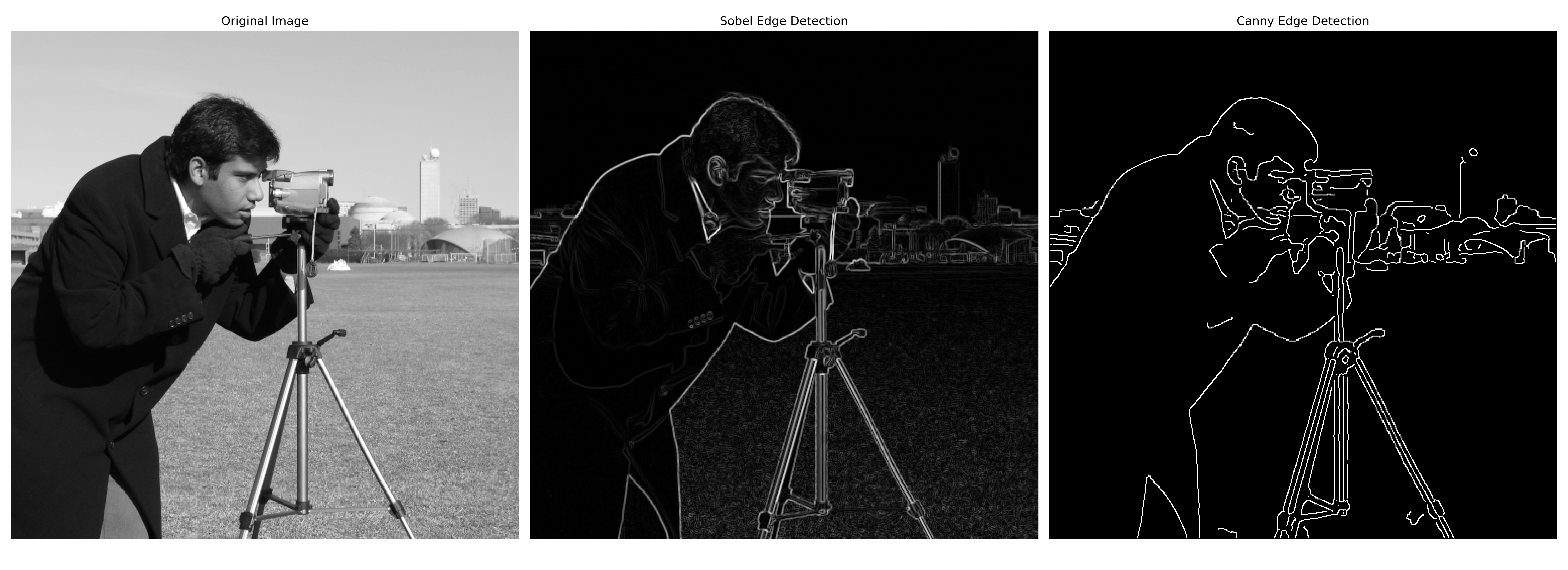

This code demonstrates two popular edge detection algorithms:

1. Sobel operator: Calculates the gradient of image intensity at each pixel, highlighting areas of rapid intensity change
2. Canny edge detector: A multi-stage algorithm that detects edges while suppressing noise

Edge detection is often one of the first steps in many computer vision pipelines, as it reduces the amount of data to process while preserving the structural information needed for further analysis.

Feature Extraction: Finding Patterns

Beyond edges, computers need to identify more complex patterns in images. This process, called feature extraction, involves identifying distinctive elements that can help in tasks like object recognition. Traditional computer vision relied heavily on hand-crafted features like:

• SIFT (Scale-Invariant Feature Transform): Identifies key points that remain consistent despite changes in scale, rotation, or illumination
• HOG (Histogram of Oriented Gradients): Counts occurrences of gradient orientation in localized portions of an image
• Haar-like features: Simple rectangular patterns used in face detection

These features provide a compact representation of the image that emphasizes the most informative parts while discarding irrelevant details.

The AI Revolution in Computer Vision

While traditional computer vision techniques laid important groundwork, the field underwent a revolutionary transformation with the rise of deep learning. Instead of relying on hand-crafted features, neural networks learn to extract relevant features directly from data.

Convolutional Neural Networks: The Game Changers

Convolutional Neural Networks (CNNs) have become the backbone of modern computer vision systems. Inspired by the organization of the animal visual cortex, CNNs apply filters across an image to detect patterns at different scales.

The CIFAR-10 Dataset: A Computer Vision Benchmark

Before diving into our code, let's explore one of the most widely used datasets in computer vision: CIFAR-10. Created by researchers at the Canadian Institute For Advanced Research, this dataset contains:

• 60,000 color images (50,000 for training, 10,000 for testing)
• 10 different classes: airplane, automobile, bird, cat, deer, dog, frog, horse, ship, and truck
• Small images of size 32×32 pixels
• Balanced classes (6,000 images per category)

This dataset has become a standard benchmark for evaluating image classification algorithms. Let's first visualize some sample images from this dataset:

import tensorflow as tf
import numpy as np
import matplotlib.pyplot as plt
import os

# Create a directory for saving figures if it doesn't exist
os.makedirs('images/blog/blog2', exist_ok=True)

# Load just a small subset of the CIFAR-10 dataset to save memory
(x_train, y_train), (x_test, y_test) = tf.keras.datasets.cifar10.load_data()
x_train = x_train[:5000]  # Just use 5000 images instead of all 50,000
y_train = y_train[:5000]

# Define class names
class_names = ['airplane', 'automobile', 'bird', 'cat', 'deer', 
               'dog', 'frog', 'horse', 'ship', 'truck']

# Print dataset statistics
print(f"Training images sample shape: {x_train.shape}")
print(f"Training labels sample shape: {y_train.shape}")
print(f"Test images shape: {x_test.shape}")
print(f"Test labels shape: {y_test.shape}")
print(f"Image dimensions: {x_train[0].shape}")
print(f"Number of classes: {len(class_names)}")
print(f"Pixel value range: {x_train.min()} to {x_train.max()}")

# Display sample images from each class
plt.figure(figsize=(12, 10))
for i in range(10):
    plt.subplot(2, 5, i+1)
    # Find the first image of each class
    idx = np.where(y_train == i)[0][0]
    plt.imshow(x_train[idx])
    plt.title(class_names[i])
    plt.axis('off')
plt.tight_layout()
plt.savefig('images/blog/blog2/cifar10_samples.png', bbox_inches='tight')
plt.show()

# Display pixel distribution with a smaller sample to save memory
sample_images = x_train[:1000]  # Just use 1000 images for the histogram
plt.figure(figsize=(15, 5))
for i, channel_name in enumerate(['Red', 'Green', 'Blue']):
    plt.subplot(1, 3, i+1)
    # Flatten sample pixel values in the channel
    channel_values = sample_images[:, :, :, i].flatten()
    plt.hist(channel_values, bins=25, alpha=0.7, color=['red', 'green', 'blue'][i])
    plt.title(f'{channel_name} Channel Distribution')
    plt.xlabel('Pixel Value')
    plt.ylabel('Frequency')
plt.tight_layout()
plt.savefig('images/blog/blog2/cifar10_pixel_distribution.png', bbox_inches='tight')
plt.show()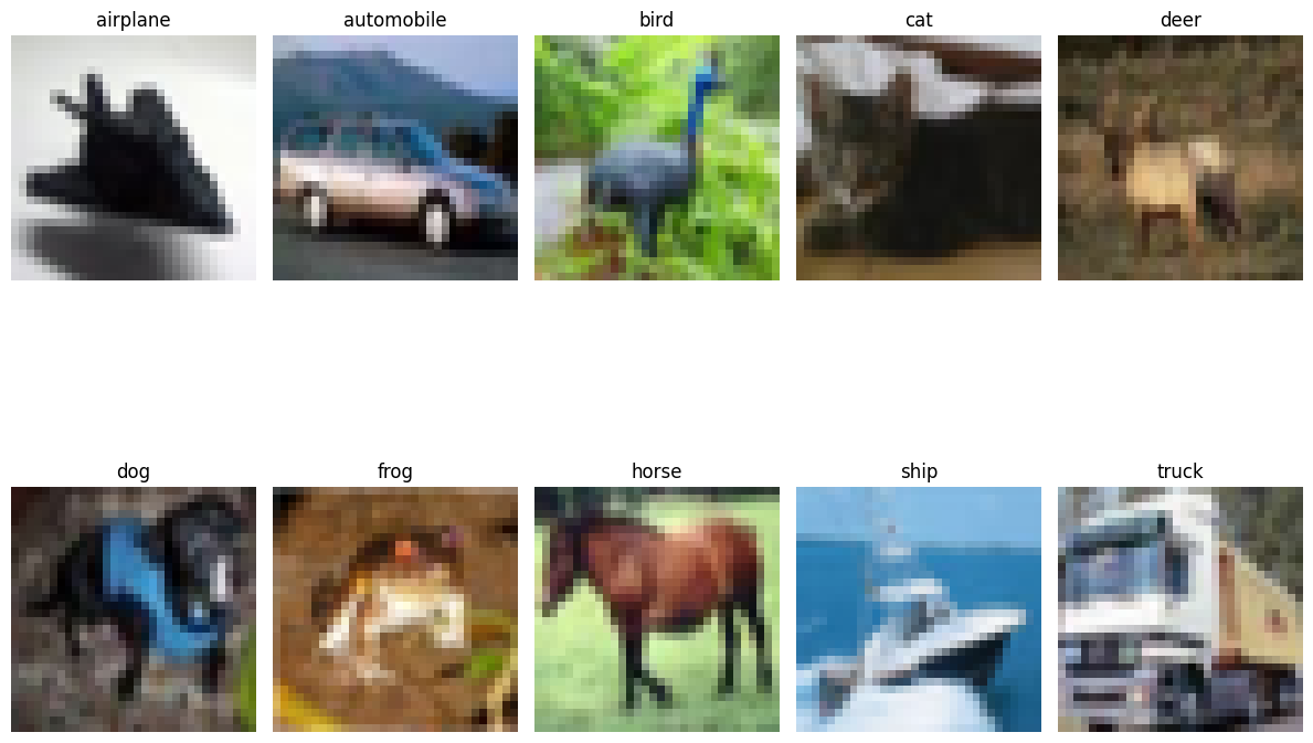

These are sample images from each of the 10 classes in the CIFAR-10 dataset. As you can see, the images are quite small (32x32 pixels) and represent common objects. Despite their small size, they contain enough information for classification algorithms to distinguish between different categories.

The histograms above show the distribution of pixel values across each color channel in the dataset. This gives us insight into the dataset's characteristics - notably, the pixels are well-distributed across the 0-255 range, with slight variations between channels.

Now, let's implement image classification using a smaller, more CPU-friendly model on a sample image:

import tensorflow as tf
import numpy as np
import matplotlib.pyplot as plt
import os
from tensorflow.keras.applications import MobileNetV2
from tensorflow.keras.applications.mobilenet_v2 import preprocess_input, decode_predictions
from tensorflow.keras.preprocessing import image
from skimage import data, transform

# Load a sample image
img = data.chelsea()  # A photo of a cat from scikit-image sample data

# Display the original image
plt.figure(figsize=(6, 6))
plt.imshow(img)
plt.title('Original Image: Chelsea the Cat')
plt.axis('off')
plt.savefig('images/blog/blog2/chelsea_original.png', bbox_inches='tight')
plt.show()

# Get image information
print(f"Image shape: {img.shape}")
print(f"Image data type: {img.dtype}")
print(f"Value range: {img.min()} to {img.max()}")

# Use a smaller image size to make processing faster (160x160 instead of 224x224)
# This is still compatible with MobileNetV2 but will use less memory
img_resized = transform.resize(img, (160, 160), anti_aliasing=True)
img_array = img_resized * 255  # Convert from [0,1] to [0,255]
img_array = img_array.astype(np.uint8)

# Display the resized image
plt.figure(figsize=(6, 6))
plt.imshow(img_array)
plt.title('Resized Image (160x160)')
plt.axis('off')
plt.savefig('images/blog/blog2/chelsea_resized.png', bbox_inches='tight')
plt.show()

# Prepare the image for the model
x = image.img_to_array(img_array)
x = np.expand_dims(x, axis=0)
x = preprocess_input(x)

# Load the pre-trained model with alpha=0.75 for a smaller, faster model
# Setting include_top=True keeps the classification head for ImageNet classes
model = MobileNetV2(weights='imagenet', input_shape=(160, 160, 3), alpha=0.75)

# Print a summary of just the first few layers to avoid a long output
print("MobileNetV2 Architecture (first few layers):")
# Only show first 5 layers in summary to keep output manageable
for i, layer in enumerate(model.layers[:5]):
    try:
        print(f"Layer {i}: {layer.name}, Output Shape: {layer.output.shape}")
    except AttributeError:
        print(f"Layer {i}: {layer.name}, Output Shape: Not Available")
    
print("...")
print(f"Total layers: {len(model.layers)}")

# Make predictions
preds = model.predict(x)
decoded_preds = decode_predictions(preds, top=5)[0]

# Create a bar chart of predictions
plt.figure(figsize=(8, 5))
classes = [pred[1].replace('_', ' ') for pred in decoded_preds]
scores = [pred[2] for pred in decoded_preds]
y_pos = np.arange(len(classes))

bars = plt.barh(y_pos, scores, align='center')
plt.yticks(y_pos, classes)
plt.xlabel('Probability')
plt.title('Top 5 Predictions')
plt.xlim(0, 1.0)

# Add percentage labels to bars
for bar in bars:
    width = bar.get_width()
    plt.text(width + 0.01, bar.get_y() + bar.get_height()/2, 
             f'{width:.2%}', ha='left', va='center')

plt.tight_layout()
plt.savefig('images/blog/blog2/chelsea_predictions.png', bbox_inches='tight')
plt.show()

# Instead of visualizing many feature maps, just show 4 to reduce computation
first_layer_model = tf.keras.Model(inputs=model.inputs, 
                                  outputs=model.get_layer('Conv1').output)
first_layer_activation = first_layer_model.predict(x)

# Display just 4 feature maps instead of 16
plt.figure(figsize=(10, 3))
for i in range(4):  # Display only 4 feature maps
    plt.subplot(1, 4, i+1)
    plt.imshow(first_layer_activation[0, :, :, i], cmap='viridis')
    plt.axis('off')
    plt.title(f'Filter {i+1}')
plt.tight_layout()
plt.savefig('images/blog/blog2/feature_maps.png', bbox_inches='tight')
plt.show()

print("Top predictions:")
for i, (imagenet_id, label, score) in enumerate(decoded_preds):
    print(f"{i+1}: {label.replace('_', ' ')} ({score:.2%})")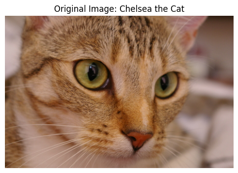

This is our input image, "Chelsea the Cat" from scikit-image's sample data collection. It's a color photograph of a tabby cat, which we'll use to test our pre-trained CNN.

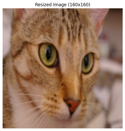
The image has been resized to 160×160 pixels to make processing faster while still providing enough detail for accurate classification.

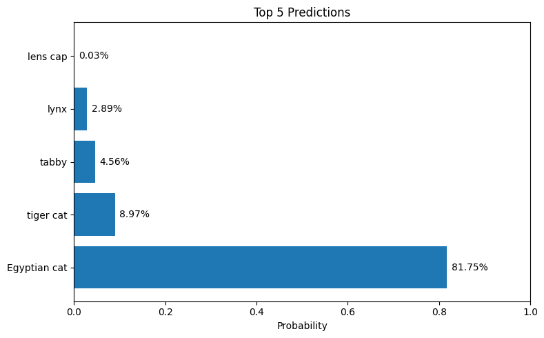
The bar chart shows the top 5 predictions made by the model. MobileNetV2 correctly identifies the image as containing a tabby cat with high confidence. The model was pre-trained on ImageNet, a dataset with over 1 million images across 1,000 classes, demonstrating how transfer learning allows us to leverage existing knowledge.

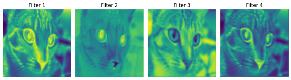
These visualizations show a sample of activation maps from the first convolutional layer of MobileNetV2. Each map represents how a specific filter responds to the input image. Some filters detect edges, others respond to textures or specific colors. These low-level features are combined in deeper layers to recognize more complex patterns.

How CNNs Work: A Peek Under the Hood

Convolutional Neural Networks consist of several types of layers:

1. Convolutional layers: Apply filters to detect features like edges, textures, and patterns
2. Pooling layers: Reduce the spatial dimensions while preserving important information
3. Fully connected layers: Combine features for final classification decisions

What makes CNNs so powerful is that they learn their own features from data, rather than relying on human-designed feature extractors. Earlier layers learn simple features like edges and corners, while deeper layers combine these to recognize complex patterns like eyes, wheels, or text.

As we saw in the feature maps visualization above, the first layer of filters detects basic visual elements. Each colored activation map shows how strongly a particular filter responds to different parts of the image. Some filters highlight edges, others respond to specific textures or color transitions. These feature detectors are not programmed explicitly—they emerge naturally through training on thousands of images.

The deeper we go into the network, the more abstract and complex these features become. Middle layers might detect combinations like "furry texture," "pointy ears," or "whiskers," while the final layers identify entire objects like "tabby cat" or "Egyptian cat." This hierarchical feature extraction is remarkably similar to how the human visual cortex processes information.

Beyond Classification: The Rich Landscape of Computer Vision Tasks

Image classification is just one of many tasks in computer vision. As the field has matured, researchers have developed specialized architectures for various applications:

Object Detection: Finding What and Where

Object detection goes beyond classification by not only identifying objects but also locating them within an image. Popular architectures include:

• YOLO (You Only Look Once): Processes the entire image in one forward pass, making it extremely fast
• Faster R-CNN: A two-stage detector that first proposes regions of interest, then classifies them
• SSD (Single Shot Detector): Balances speed and accuracy by making predictions at multiple scales

Semantic Segmentation: Understanding Every Pixel

While object detection draws boxes around objects, semantic segmentation classifies every pixel in an image. This allows for precise delineation of object boundaries:

"If classification asks 'what is in this image?' and detection asks 'what and where?', then segmentation asks 'what is the category of each pixel?'"

Image Generation and Manipulation

Perhaps the most remarkable recent developments have been in generative models that can create or modify images:

• GANs (Generative Adversarial Networks): Two neural networks compete, with one generating images and the other judging their authenticity
• Diffusion Models: Gradually add and then remove noise to generate high-quality images
• Style Transfer: Apply the artistic style of one image to the content of another

The Human-Machine Vision Gap

Despite tremendous advances, computer vision systems still differ fundamentally from human vision in several ways:

• Context understanding: Humans excel at using context to resolve ambiguities
• Generalization ability: We can recognize objects from novel viewpoints or in unusual settings
• Common sense reasoning: We understand physical constraints and relationships
• Intentionality detection: We can infer goals and intentions from visual cues

These differences highlight both the limitations of current systems and the exciting research directions still to be explored.

Real-World Applications: Vision in Action

The theoretical foundations of computer vision enable countless practical applications:

• Healthcare: Analyzing medical images to detect diseases from cancer to diabetic retinopathy
• Autonomous vehicles: Helping cars perceive their environment and make driving decisions
• Augmented reality: Overlaying digital content onto the physical world
• Security and surveillance: Identifying suspicious activities or unauthorized access
• Retail: Enabling cashierless stores and inventory management
• Agriculture: Monitoring crop health and optimizing harvests

Each of these applications combines multiple computer vision techniques, often integrating them with other AI components like natural language processing or reinforcement learning.

Looking Forward: The Future of Computer Vision

As we continue to develop more sophisticated vision systems, several trends are shaping the future of the field:

Multimodal Understanding

Future systems will increasingly integrate vision with other modalities like language, audio, and tactile information—much as humans use multiple senses to understand the world.

Self-Supervised Learning

Moving beyond human-labeled datasets, self-supervised learning allows models to learn from the internal structure of images, greatly reducing the need for annotated data.

Ethical Considerations

As vision systems become more pervasive, addressing issues of privacy, bias, and security becomes increasingly important. The images used to train models may contain unintended biases that affect system performance across different demographic groups.

Energy Efficiency

Developing more efficient architectures will be crucial for deploying vision systems on edge devices with limited computational resources.

Final Thoughts: Bridging Two Worlds of Vision

Computer vision represents one of humanity's most ambitious projects: teaching machines to interpret the visual world. While the pixels-and-algorithms approach differs fundamentally from our biological vision system, the parallels are striking. Both transform raw visual data into increasingly abstract representations that support understanding and action.

As computer vision continues to evolve, the gap between human and machine perception may narrow—not because machines will see exactly as we do, but because they'll develop their own powerful ways of extracting meaning from images. This collaboration between human and artificial intelligence opens possibilities that neither could achieve alone.

The next time you unlock your phone with your face, search for images without text, or watch an autonomous vehicle navigate traffic, take a moment to appreciate the remarkable journey from pixels to understanding that makes these technologies possible.

And perhaps most fascinating of all: our efforts to teach machines to see have taught us more about our own vision—how we perceive depth, recognize patterns, and construct meaning from light. In building artificial vision, we've gained new insights into one of nature's most remarkable creations: the human visual system.