Beyond Labels: How Machines Learn to See With and Without Human Guidance

Have you ever watched a child learn to recognize objects? Initially, parents point and name things directly: "That's a cat", "This is an apple". But soon, the child learns independently, categorizing new objects without explicit instruction. This beautiful transition from guided to autonomous learning mirrors one of the most fascinating aspects of artificial intelligence: the spectrum of learning paradigms.

In the realm of computer vision, machines can learn in remarkably different ways—from the meticulously hand-labeled datasets of supervised learning to the autonomous pattern discovery of unsupervised approaches. Each method offers unique insights into both machine and human cognition, revealing different paths to visual understanding.

This journey through learning paradigms isn't just about technical approaches; it's about fundamental questions of knowledge acquisition. How much guidance do machines need? Can they discover meaningful patterns independently? What parallels exist between machine learning and human visual development?

Let's explore this landscape of learning paradigms and discover how each shapes the way machines perceive and understand our visual world.

The Spectrum of Learning: From Full Guidance to Complete Autonomy

Machine learning approaches in computer vision span a continuum from fully guided to completely autonomous:

Supervised → Semi-Supervised → Self-Supervised → Unsupervised → Reinforcement Learning
(Most Guided) ----------------------------------------> (Most Autonomous)

Each paradigm represents a different balance of human guidance and machine independence, with unique strengths and limitations. Let's begin our exploration with the most guided approach.

Supervised Learning: Learning from Human Teachers

Supervised learning is the most straightforward approach: humans provide labeled examples, and machines learn to recognize patterns that connect inputs to outputs. It's analogous to a teacher showing flashcards to a student, providing both the question (image) and the answer (label).

"Supervised learning is the computational equivalent of learning with a patient teacher who shows you examples and tells you the right answer every time."

The MNIST Dataset: A Classic Teaching Tool

To understand supervised learning in practice, let's start with the classic MNIST dataset—a collection of handwritten digits that has served as a training ground for image classification algorithms for decades.

import numpy as np
import matplotlib.pyplot as plt
from sklearn.datasets import fetch_openml
from sklearn.model_selection import train_test_split
from sklearn.linear_model import LogisticRegression
from sklearn.metrics import accuracy_score, confusion_matrix
import seaborn as sns
import os

# Create directory for saving generated images
os.makedirs('images/blog/learning_paradigms', exist_ok=True)

# Load a subset of MNIST data (using a smaller subset to be CPU-friendly)
print("Loading MNIST data...")
X, y = fetch_openml('mnist_784', version=1, return_X_y=True, as_frame=False, parser='auto')
X = X / 255.0  # Normalize pixel values

# Use only a subset of the data to keep it CPU-friendly
n_samples = 5000
X = X[:n_samples]
y = y[:n_samples]

# Split the data
X_train, X_test, y_train, y_test = train_test_split(X, y, test_size=0.2, random_state=42)

print(f"Training on {X_train.shape[0]} samples, testing on {X_test.shape[0]} samples")

# Display a few examples
plt.figure(figsize=(12, 5))
for i in range(10):
    plt.subplot(2, 5, i+1)
    plt.imshow(X_train[i].reshape(28, 28), cmap='gray')
    plt.title(f"Label: {y_train[i]}")
    plt.axis('off')
plt.tight_layout()
plt.savefig('images/blog/learning_paradigms/mnist_examples.png')
plt.close()

# Train a simple model (Logistic Regression is CPU-friendly)
print("Training logistic regression model...")
clf = LogisticRegression(max_iter=100, solver='saga', tol=0.1)
clf.fit(X_train, y_train)

# Make predictions
y_pred = clf.predict(X_test)
accuracy = accuracy_score(y_test, y_pred)
print(f"Accuracy: {accuracy:.4f}")

# Create confusion matrix
cm = confusion_matrix(y_test, y_pred)

# Plot confusion matrix
plt.figure(figsize=(10, 8))
sns.heatmap(cm, annot=True, fmt='d', cmap='Blues')
plt.xlabel('Predicted Labels')
plt.ylabel('True Labels')
plt.title('Confusion Matrix')
plt.savefig('images/blog/learning_paradigms/confusion_matrix.png')
plt.close()

# Show some predictions
plt.figure(figsize=(12, 8))
for i in range(15):
    plt.subplot(3, 5, i+1)
    plt.imshow(X_test[i].reshape(28, 28), cmap='gray')
    pred = clf.predict([X_test[i]])[0]
    true = y_test[i]
    color = 'green' if pred == true else 'red'
    plt.title(f"Pred: {pred}\nTrue: {true}", color=color)
    plt.axis('off')
plt.tight_layout()
plt.savefig('images/blog/learning_paradigms/predictions.png')
plt.close()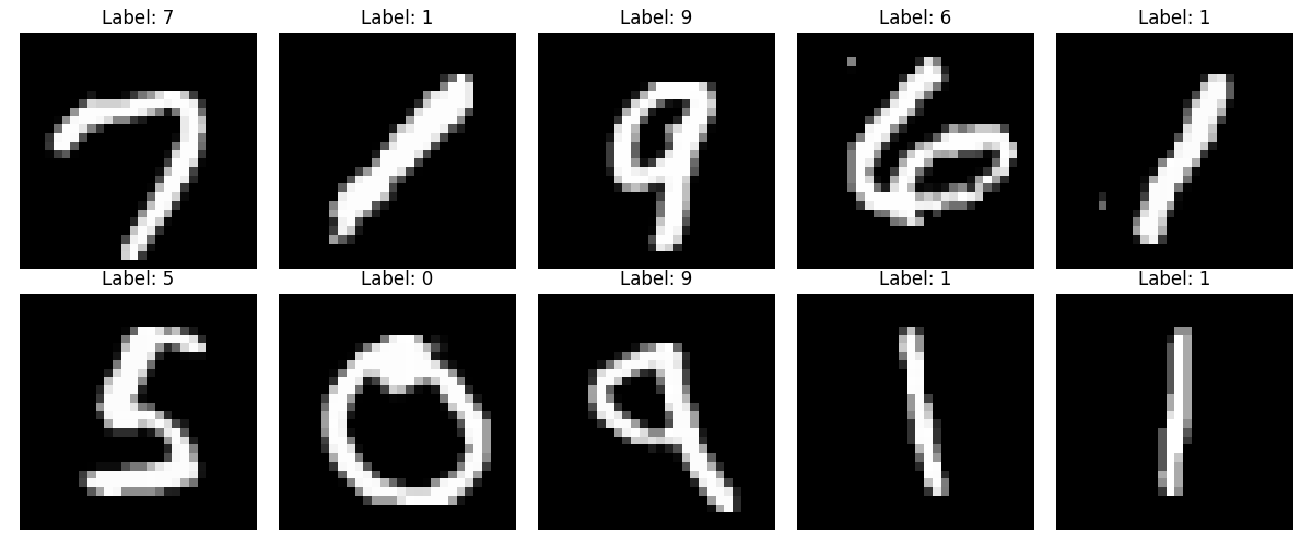

In this example, we've loaded a subset of the MNIST dataset and displayed some sample images with their corresponding labels. Each image is a 28×28 pixel grayscale representation of a handwritten digit, and each comes with a label indicating which digit it represents (0-9).

This perfectly exemplifies supervised learning: the dataset provides both the input (image) and the expected output (digit label). Our algorithm's task is to learn the mapping between the visual patterns and their corresponding digits.

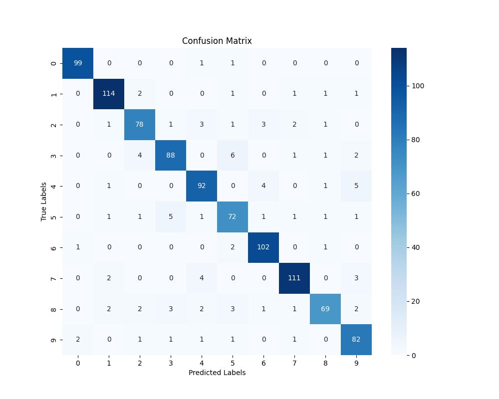
The confusion matrix above visualizes our model's performance. Each cell shows how many images of a true digit (rows) were classified as each predicted digit (columns). The diagonal represents correct classifications, while off-diagonal elements show errors. For example, we can see that the model occasionally confuses '4' with '9', which makes intuitive sense given their visual similarities.

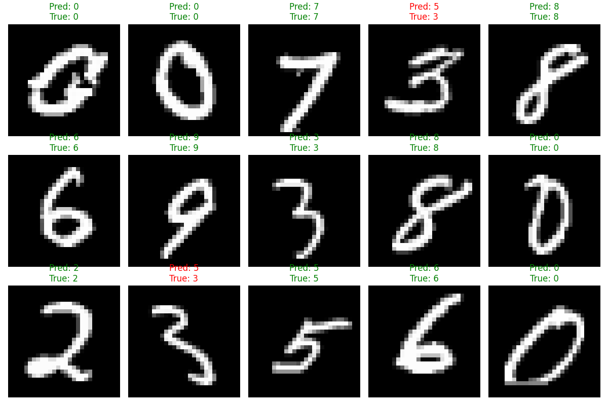
Here we see some test examples with both the true label and our model's prediction. Green titles indicate correct predictions, while red shows mistakes. Even with a relatively simple logistic regression model, we achieve good accuracy on this task.

The Power and Limitations of Supervision

Supervised learning excels when:

• We have a clear definition of what we're looking for
• We can provide many labeled examples
• The test data is similar to the training data

However, it faces significant challenges:

• Label dependency: Performance is only as good as your labels
• Data hunger: Requires large amounts of labeled data
• Generalization gap: Often struggles with novel scenarios
• Label bias: Models inherit biases present in the labeling process

These limitations have pushed researchers to explore less supervised approaches, which we'll examine next.

Unsupervised Learning: Finding Patterns Without Guidance

At the opposite end of the spectrum is unsupervised learning, where algorithms receive data without any labels. The goal shifts from mapping inputs to outputs to discovering inherent structure within the data itself. It's like giving a child a box of varied objects and watching them sort them based on their own observed similarities.

"Unsupervised learning is the computational equivalent of exploring a new territory without a map, where you must discover the landmarks and pathways yourself."

Clustering Images: Discovering Visual Categories

One of the most common unsupervised learning techniques is clustering. Let's see how we can use clustering to discover natural groupings in image data:

import numpy as np
import matplotlib.pyplot as plt
from sklearn.datasets import fetch_olivetti_faces
from sklearn.cluster import KMeans
from sklearn.decomposition import PCA
import os

# Load the Olivetti faces dataset (small enough for CPU)
faces = fetch_olivetti_faces(shuffle=True)
X = faces.data
y = faces.target

print(f"Dataset shape: {X.shape}")
print(f"Number of unique individuals: {len(np.unique(y))}")

# Display some sample faces
plt.figure(figsize=(12, 8))
for i in range(15):
    plt.subplot(3, 5, i+1)
    plt.imshow(X[i].reshape(64, 64), cmap='gray')
    plt.title(f"Person: {y[i]}")
    plt.axis('off')
plt.tight_layout()
plt.savefig('images/blog/learning_paradigms/sample_faces.png')
plt.close()

# Apply dimensionality reduction for visualization
pca = PCA(n_components=2)
X_pca = pca.fit_transform(X)

# Apply K-means clustering (unsupervised)
n_clusters = 10  # We'll try to find 10 clusters
kmeans = KMeans(n_clusters=n_clusters, random_state=42, n_init=10)
clusters = kmeans.fit_predict(X)

# Visualize the clusters in 2D space
plt.figure(figsize=(10, 8))
scatter = plt.scatter(X_pca[:, 0], X_pca[:, 1], c=clusters, cmap='viridis', 
                     alpha=0.7, s=50, edgecolors='w')
centers = pca.transform(kmeans.cluster_centers_)
plt.scatter(centers[:, 0], centers[:, 1], c='red', s=200, alpha=0.5, marker='X')
plt.title('Face Images Clustered in 2D Space')
plt.xlabel('Principal Component 1')
plt.ylabel('Principal Component 2')
plt.colorbar(scatter, label='Cluster')
plt.savefig('images/blog/learning_paradigms/face_clusters_2d.png')
plt.close()

# Display representative faces from each cluster
plt.figure(figsize=(15, 8))
for i in range(n_clusters):
    cluster_examples = np.where(clusters == i)[0][:5]  # Get first 5 examples from cluster
    for j, idx in enumerate(cluster_examples[:min(5, len(cluster_examples))]):
        plt.subplot(n_clusters, 5, i*5 + j + 1)
        plt.imshow(X[idx].reshape(64, 64), cmap='gray')
        plt.title(f"C{i}: P{y[idx]}")
        plt.axis('off')
plt.tight_layout()
plt.savefig('images/blog/learning_paradigms/cluster_representatives.png')
plt.close()

# Compare clusters with true identities
cluster_to_person = {}
for cluster in range(n_clusters):
    cluster_samples = np.where(clusters == cluster)[0]
    person_counts = np.bincount(y[cluster_samples])
    main_person = np.argmax(person_counts)
    purity = person_counts[main_person] / len(cluster_samples)
    cluster_to_person[cluster] = (main_person, purity)
    print(f"Cluster {cluster}: Mainly person {main_person} (purity: {purity:.2f})")

# Visualize cluster purity
clusters_list = list(range(n_clusters))
purities = [cluster_to_person[c][1] for c in clusters_list]
plt.figure(figsize=(10, 6))
bars = plt.bar(clusters_list, purities, color='skyblue')
plt.axhline(y=0.5, color='r', linestyle='--', alpha=0.7)
plt.xlabel('Cluster')
plt.ylabel('Purity (Ratio of Dominant Person)')
plt.title('How Well Do Clusters Capture Individual Identities?')
plt.ylim(0, 1.0)
plt.xticks(clusters_list)

# Add value labels to bars
for bar in bars:
    height = bar.get_height()
    plt.text(bar.get_x() + bar.get_width()/2., height + 0.02,
             f'{height:.2f}', ha='center', va='bottom')

plt.tight_layout()
plt.savefig('images/blog/learning_paradigms/cluster_purity.png')
plt.close()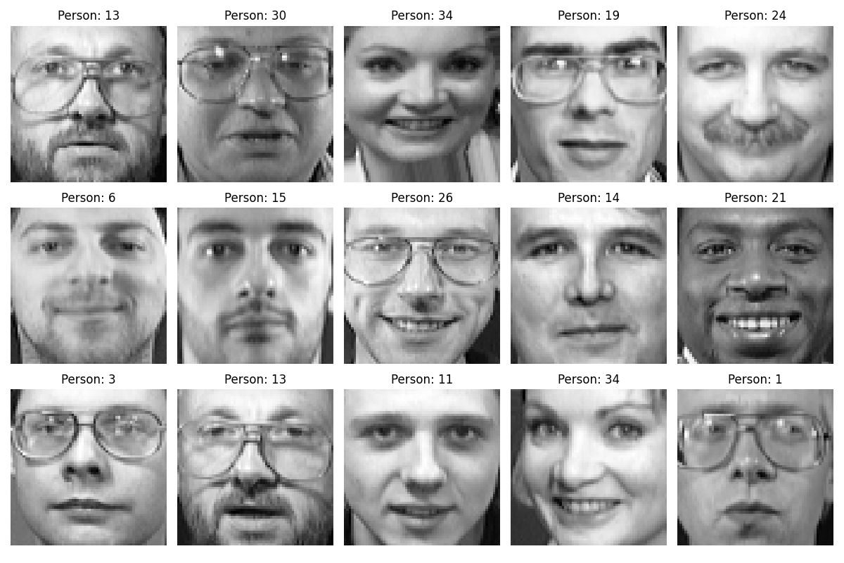

Here we see sample faces from the Olivetti dataset, which contains 400 images of 40 different individuals. Each image is 64×64 pixels in grayscale. Unlike MNIST, we're going to pretend we don't have the identity labels and see if our unsupervised algorithm can discover natural groupings.

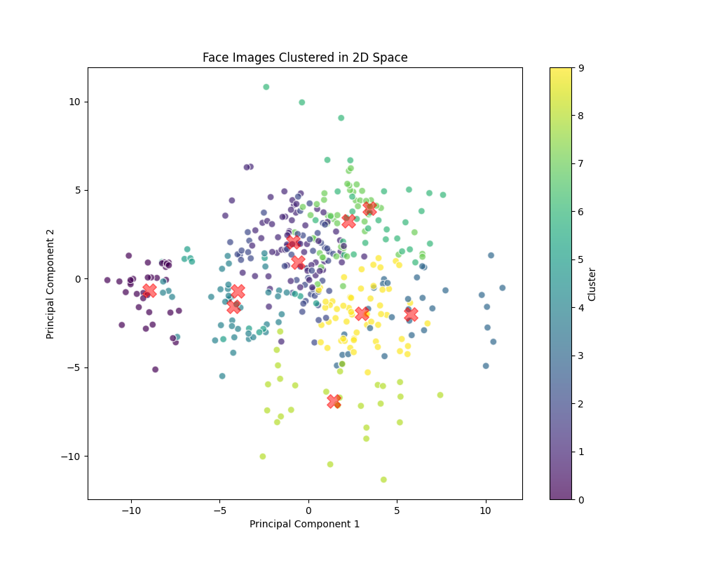
This visualization shows our facial images projected into a 2D space using Principal Component Analysis (PCA), with colors indicating the clusters discovered by the K-means algorithm. Each point represents a face image, and points with the same color were grouped together based on visual similarity—without any knowledge of the actual identities.

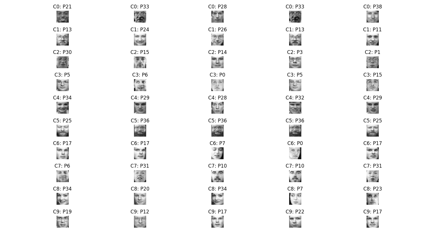
Here we see representative faces from each of our discovered clusters. Notice how many clusters contain multiple images of the same person, even though we never explicitly told the algorithm about identities. The algorithm has independently discovered that images of the same person tend to be visually similar.

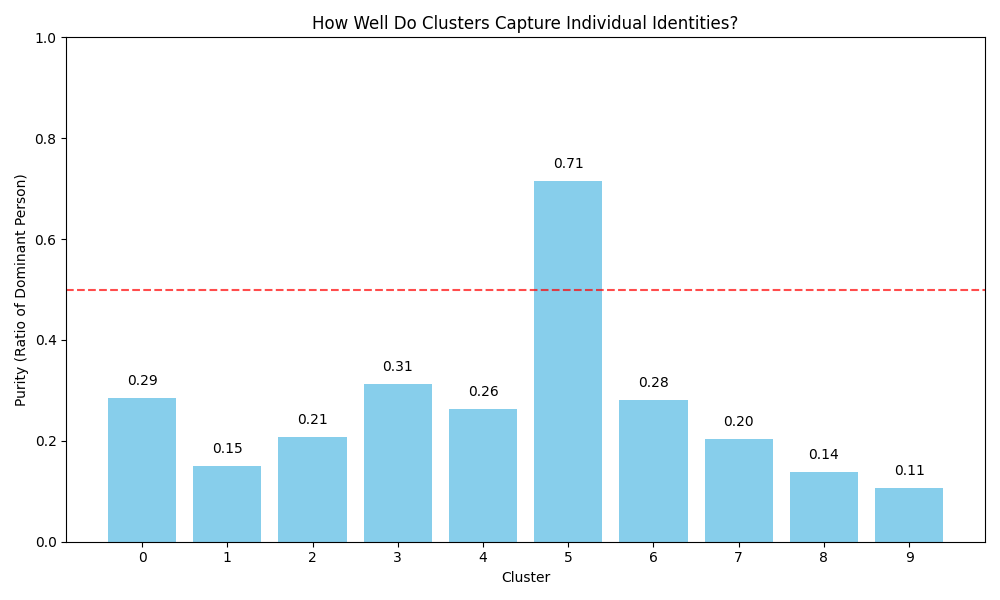
This chart shows the "purity" of each cluster—what percentage of images in the cluster belong to the most common person in that cluster. Higher values indicate that the cluster mainly contains a single individual. Some clusters have achieved impressive purity, showing that K-means has discovered meaningful groupings that align with actual identities, despite never being trained on identity labels.

Dimensionality Reduction: Visualizing High-Dimensional Data

Another key unsupervised technique is dimensionality reduction, which helps us visualize and understand complex high-dimensional data like images. Let's explore how PCA and t-SNE can reveal structure in image data:

import numpy as np
import matplotlib.pyplot as plt
from sklearn.datasets import fetch_openml
from sklearn.decomposition import PCA
from sklearn.manifold import TSNE
import time

# Load a subset of MNIST data again
X, y = fetch_openml('mnist_784', version=1, return_X_y=True, as_frame=False, parser='auto')
X = X / 255.0

# Use a small subset to keep it CPU-friendly
n_samples = 2000
X_subset = X[:n_samples]
y_subset = y[:n_samples]

print(f"Working with {n_samples} samples")

# Apply PCA
n_components = 50
print("Applying PCA...")
pca = PCA(n_components=n_components)
X_pca = pca.fit_transform(X_subset)

# Plot explained variance
plt.figure(figsize=(10, 6))
explained_variance = pca.explained_variance_ratio_
cumulative_variance = np.cumsum(explained_variance)
plt.bar(range(1, n_components+1), explained_variance, alpha=0.7, color='skyblue', 
        label='Individual Component')
plt.step(range(1, n_components+1), cumulative_variance, where='mid', color='red', 
         label='Cumulative Explained Variance')
plt.axhline(y=0.9, color='green', linestyle='--', alpha=0.5, label='90% Explained Variance')
plt.xlabel('Principal Component')
plt.ylabel('Explained Variance Ratio')
plt.title('Explained Variance by Principal Components')
plt.legend()
plt.grid(alpha=0.3)
plt.tight_layout()
plt.savefig('images/blog/learning_paradigms/pca_explained_variance.png')
plt.close()

# Apply t-SNE (on PCA results for speed)
print("Applying t-SNE (this might take a minute)...")
start_time = time.time()
tsne = TSNE(n_components=2, perplexity=30, learning_rate=200, random_state=42, 
           init='pca')
X_tsne = tsne.fit_transform(X_pca)
print(f"t-SNE completed in {time.time() - start_time:.2f} seconds")

# Plot t-SNE results
plt.figure(figsize=(12, 10))
scatter = plt.scatter(X_tsne[:, 0], X_tsne[:, 1], c=y_subset.astype(int), 
                     cmap='tab10', alpha=0.7, s=50, edgecolors='w')
plt.colorbar(scatter, label='Digit')
plt.title('t-SNE Visualization of MNIST Digits')
plt.xlabel('t-SNE Dimension 1')
plt.ylabel('t-SNE Dimension 2')
plt.grid(alpha=0.3)
plt.tight_layout()
plt.savefig('images/blog/learning_paradigms/tsne_visualization.png')
plt.close()

# Visualize some reconstructed digits with PCA
n_display = 5
plt.figure(figsize=(15, 4))
for i in range(n_display):
    # Original image
    plt.subplot(2, n_display, i+1)
    plt.imshow(X_subset[i].reshape(28, 28), cmap='gray')
    plt.title(f"Original: {y_subset[i]}")
    plt.axis('off')
    
    # Reconstructed image
    plt.subplot(2, n_display, i+1+n_display)
    X_reconstructed = pca.inverse_transform(X_pca[i]).reshape(28, 28)
    plt.imshow(X_reconstructed, cmap='gray')
    plt.title(f"PCA Reconstructed\n({n_components} components)")
    plt.axis('off')
plt.tight_layout()
plt.savefig('images/blog/learning_paradigms/pca_reconstruction.png')
plt.close()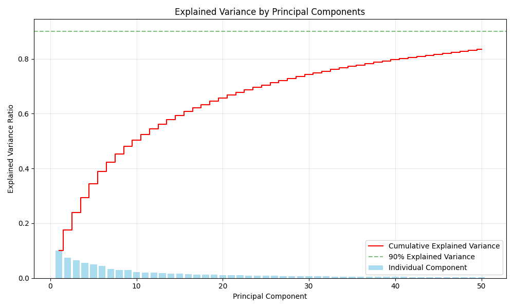

This chart shows how much information is retained by each principal component. The blue bars represent the variance explained by individual components, while the red line shows the cumulative explained variance. We can see that with just 30-40 components, we capture over 90% of the information in the original 784-dimensional images (28×28 = 784 pixels).

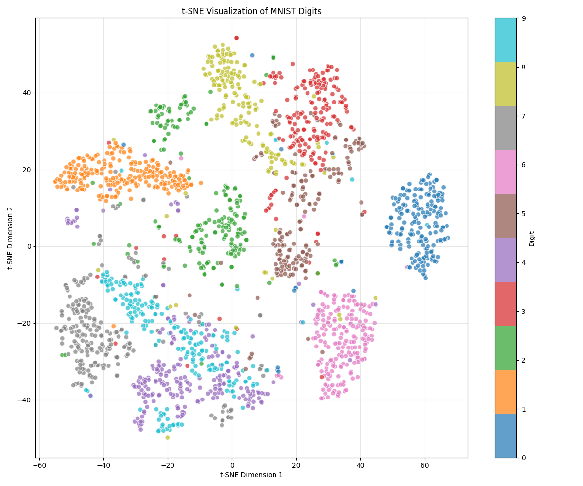
t-SNE (t-Distributed Stochastic Neighbor Embedding) is a powerful dimensionality reduction technique that preserves local structures in the data. Here, we've projected our MNIST digits into a 2D space where similar digits cluster together. Even though t-SNE wasn't given any digit labels, it naturally separated the different digit classes based on visual similarity. Notice how most digits form distinct clusters, with some expected confusion (like between 4s and 9s).

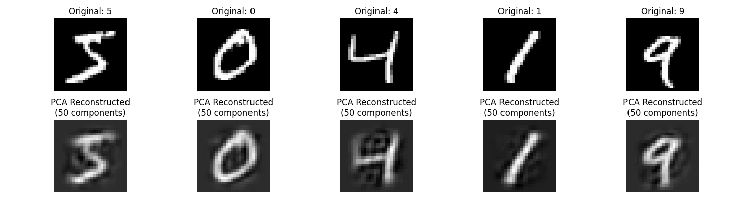
Here we demonstrate image reconstruction using PCA. The top row shows original images, while the bottom row shows reconstructions using just 50 principal components (instead of the original 784 dimensions). Even with this significant dimensionality reduction, the reconstructions preserve the essential characteristics of the digits, showing that PCA has captured the most important visual patterns.

The Power and Limitations of Unsupervised Learning

Unsupervised learning offers unique advantages:

• No labeling required: Works with raw, unlabeled data
• Pattern discovery: Can find unexpected structures and relationships
• Feature learning: Creates useful representations for downstream tasks

However, it also has significant challenges:

• Evaluation difficulty: Hard to objectively measure success
• Interpretation challenges: Discovered patterns may not align with human-meaningful categories
• Computational intensity: Many algorithms are resource-intensive

These complementary strengths and weaknesses of supervised and unsupervised learning have led to hybrid approaches that try to get the best of both worlds.

Semi-Supervised Learning: Making the Most of Limited Labels

In real-world scenarios, we often have a small amount of labeled data and a large pool of unlabeled data. Semi-supervised learning leverages both, using the labeled examples to guide learning while extracting additional patterns from the unlabeled data.

"Semi-supervised learning is like having a teacher who gives you a few examples but then encourages you to explore and learn from many more unlabeled cases on your own."

Let's implement a basic semi-supervised learning approach using a technique called Self-Training:

import numpy as np
import matplotlib.pyplot as plt
from sklearn.datasets import fetch_openml
from sklearn.semi_supervised import SelfTrainingClassifier
from sklearn.svm import SVC
from sklearn.metrics import accuracy_score
from sklearn.model_selection import train_test_split

# Load MNIST data (subset)
X, y = fetch_openml('mnist_784', version=1, return_X_y=True, as_frame=False, parser='auto')
X = X / 255.0  # Normalize

# Use a smaller subset to keep it CPU-friendly
n_samples = 3000
X = X[:n_samples]
y = y[:n_samples]

# Split into training and test sets
X_train, X_test, y_train, y_test = train_test_split(X, y, test_size=0.2, random_state=42)

# We'll simulate having limited labeled data by "hiding" most labels
labeled_ratio = 0.1  # Only 10% of training data will have labels
n_labeled = int(labeled_ratio * len(X_train))

# Create a mask for labeled data
labeled_mask = np.zeros(len(y_train), dtype=bool)
labeled_mask[:n_labeled] = True
np.random.shuffle(labeled_mask)

# Create partially labeled training data
y_train_partial = np.array(y_train)
# Replace labels for unlabeled data with -1 (the convention for unlabeled data)
y_train_partial[~labeled_mask] = -1

print(f"Total training samples: {len(X_train)}")
print(f"Labeled samples: {sum(labeled_mask)} ({labeled_ratio:.0%})")
print(f"Unlabeled samples: {sum(~labeled_mask)} ({1-labeled_ratio:.0%})")

# Create a base classifier - use LinearSVC for speed on CPU
base_clf = SVC(kernel='linear', probability=True, gamma='auto', C=1)

# Create a self-training classifier
self_training_clf = SelfTrainingClassifier(
    base_clf, threshold=0.75, max_iter=5, verbose=True
)

# Train with partially labeled data
print("Training semi-supervised model...")
self_training_clf.fit(X_train, y_train_partial)

# For comparison, train a regular model using only labeled data
print("Training supervised model with only labeled data...")
supervised_clf = SVC(kernel='linear', probability=True, gamma='auto', C=1)
supervised_clf.fit(X_train[labeled_mask], y_train[labeled_mask])

# Evaluate both models
y_pred_semi = self_training_clf.predict(X_test)
y_pred_supervised = supervised_clf.predict(X_test)

acc_semi = accuracy_score(y_test, y_pred_semi)
acc_supervised = accuracy_score(y_test, y_pred_supervised)

print(f"Semi-supervised accuracy: {acc_semi:.4f}")
print(f"Supervised-only accuracy: {acc_supervised:.4f}")
print(f"Improvement: {(acc_semi - acc_supervised) * 100:.2f} percentage points")

# Plot comparison
plt.figure(figsize=(10, 6))
models = ['Supervised\n(10% labeled)', 'Semi-Supervised\n(10% labeled + 90% unlabeled)']
accuracies = [acc_supervised, acc_semi]
bars = plt.bar(models, accuracies, color=['skyblue', 'mediumseagreen'])
plt.ylabel('Test Accuracy')
plt.title('Semi-Supervised vs. Supervised Learning with Limited Labels')
plt.ylim(0, 1.0)

# Add value labels to bars
for bar in bars:
    height = bar.get_height()
    plt.text(bar.get_x() + bar.get_width()/2., height + 0.01,
             f'{height:.3f}', ha='center', va='bottom')

plt.grid(axis='y', alpha=0.3)
plt.tight_layout()
plt.savefig('images/blog/learning_paradigms/semi_supervised_comparison.png')
plt.close()

# Visualize some test examples with predictions from both models
n_display = 15
plt.figure(figsize=(15, 8))
for i in range(n_display):
    plt.subplot(3, 5, i+1)
    plt.imshow(X_test[i].reshape(28, 28), cmap='gray')
    
    # Get predictions
    semi_pred = self_training_clf.predict([X_test[i]])[0]
    sup_pred = supervised_clf.predict([X_test[i]])[0]
    true_label = y_test[i]
    
    # Set title color based on correctness
    semi_color = 'green' if semi_pred == true_label else 'red'
    sup_color = 'green' if sup_pred == true_label else 'red'
    
    plt.title(f"True: {true_label}\nSemi: {semi_pred} ({semi_color})\nSup: {sup_pred} ({sup_color})")
    plt.axis('off')
plt.tight_layout()
plt.savefig('images/blog/learning_paradigms/semi_supervised_predictions.png')
plt.close()

# Visualize the learning curve - how performance improves with more unlabeled data
label_ratios = [0.05, 0.1, 0.2, 0.3, 0.5, 1.0]
semi_accuracies = []
supervised_accuracies = []

for ratio in label_ratios:
    if ratio == 1.0:
        # If using all data as labeled, both methods are the same
        n_labeled = len(X_train)
        labeled_mask = np.ones(len(y_train), dtype=bool)
    else:
        n_labeled = int(ratio * len(X_train))
        labeled_mask = np.zeros(len(y_train), dtype=bool)
        labeled_mask[:n_labeled] = True
        np.random.shuffle(labeled_mask)
    
    y_train_partial = np.array(y_train)
    y_train_partial[~labeled_mask] = -1
    
    # Train supervised model on labeled data only
    supervised_clf = SVC(kernel='linear', probability=True, gamma='auto', C=1)
    supervised_clf.fit(X_train[labeled_mask], y_train[labeled_mask])
    
    # For the fully labeled case, skip self-training (it would be the same)
    if ratio == 1.0:
        semi_clf = supervised_clf
    else:
        # Train semi-supervised model
        base_clf = SVC(kernel='linear', probability=True, gamma='auto', C=1)
        semi_clf = SelfTrainingClassifier(base_clf, threshold=0.75, max_iter=5)
        semi_clf.fit(X_train, y_train_partial)
    
    # Evaluate
    semi_acc = accuracy_score(y_test, semi_clf.predict(X_test))
    sup_acc = accuracy_score(y_test, supervised_clf.predict(X_test))
    
    semi_accuracies.append(semi_acc)
    supervised_accuracies.append(sup_acc)
    
    print(f"Ratio {ratio:.0%}: Semi-supervised: {semi_acc:.4f}, Supervised: {sup_acc:.4f}")

# Plot learning curve
plt.figure(figsize=(10, 6))
plt.plot(label_ratios, supervised_accuracies, 'o-', color='skyblue', label='Supervised Only')
plt.plot(label_ratios, semi_accuracies, 'o-', color='mediumseagreen', label='Semi-Supervised')
plt.xlabel('Proportion of Labeled Training Data')
plt.ylabel('Test Accuracy')
plt.title('Learning Curves: How Performance Scales with Labeled Data')
plt.grid(alpha=0.3)
plt.legend()
x_labels = [f"{int(r*100)}%" for r in label_ratios]
plt.xticks(label_ratios, x_labels)
plt.tight_layout()
plt.savefig('images/blog/learning_paradigms/learning_curves.png')
plt.close()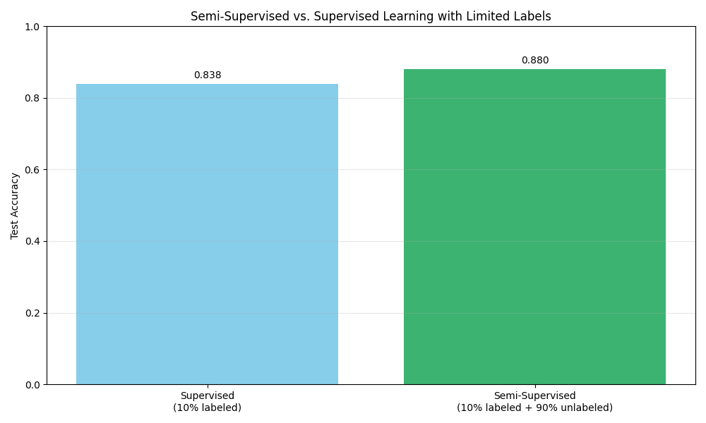

This bar chart compares the performance of a purely supervised model (trained on just 10% of labeled data) with a semi-supervised model (trained on the same 10% labeled data plus the remaining 90% of unlabeled data). We can see that leveraging the unlabeled data through self-training improves classification accuracy.

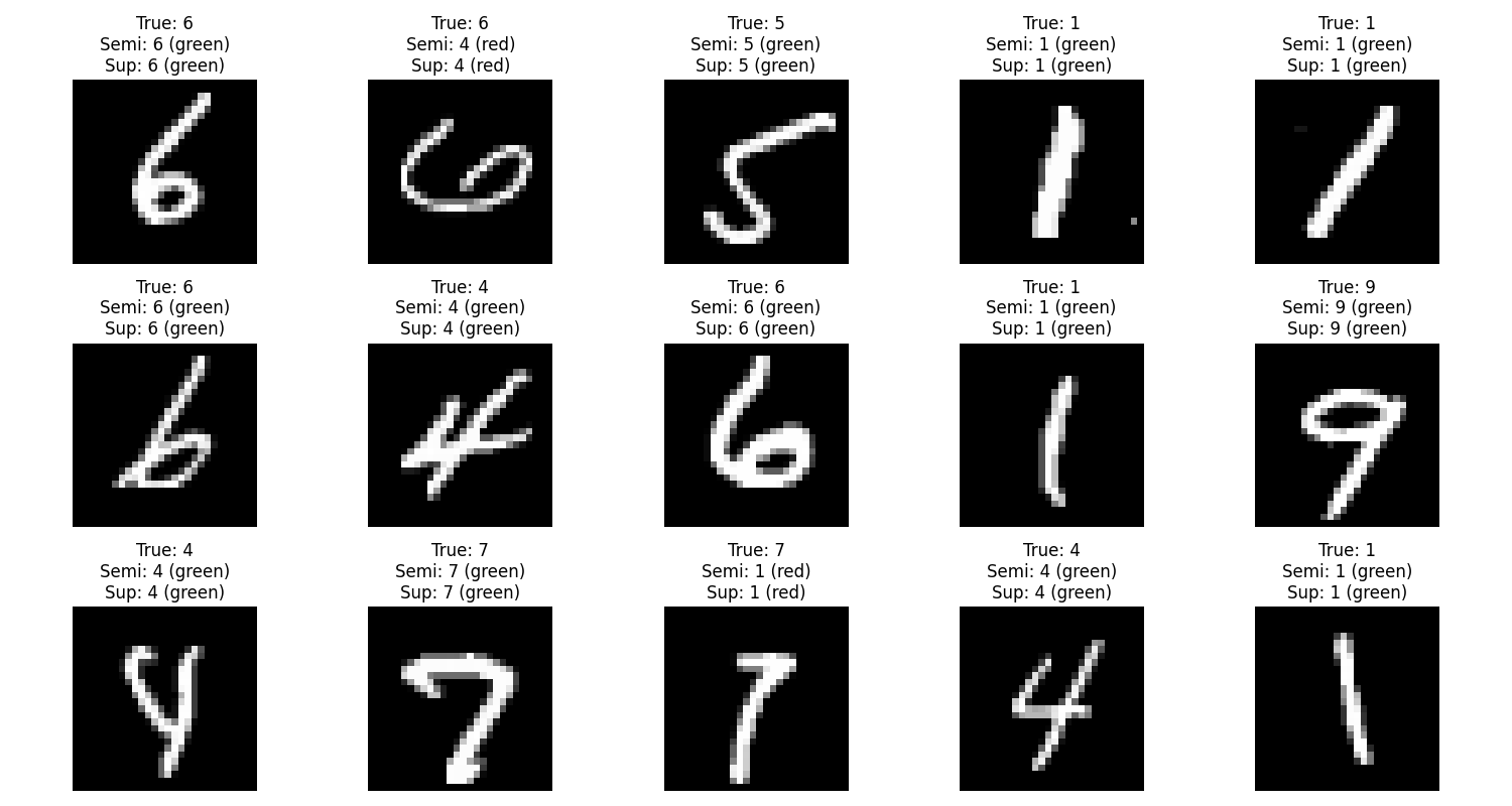
Here we see test examples with predictions from both models. Green indicates correct predictions, while red indicates errors. In several cases, the semi-supervised model correctly classifies digits that the supervised-only model gets wrong, demonstrating how the additional unlabeled data helps refine the decision boundaries.

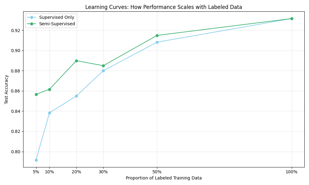
This learning curve shows how performance scales with the proportion of labeled data. The semi-supervised approach (green) consistently outperforms the supervised-only approach (blue) when labeled data is limited. As the proportion of labeled data increases, the gap narrows until they converge when all data is labeled. This illustrates a key advantage of semi-supervised learning: getting better performance when labels are scarce.

How Self-Training Works

The self-training algorithm we used follows a simple but effective approach:

1. Train an initial model on the labeled data
2. Use this model to make predictions on unlabeled data
3. Add the most confident predictions (above a threshold) to the labeled set
4. Retrain the model with the expanded labeled set
5. Repeat until convergence or for a fixed number of iterations

This iterative process leverages the model's own confident predictions to gradually expand its knowledge, similar to how a student might start with basic examples from a teacher and then practice independently on unlabeled problems.

Self-Supervised Learning: Teaching Machines to Teach Themselves

Self-supervised learning represents one of the most exciting recent developments in machine learning. Unlike unsupervised learning, which typically aims to discover any structure in data, self-supervised learning creates specific "pretext tasks" where the data provides its own supervision.

"In self-supervised learning, the data becomes its own teacher. The algorithm learns to predict one part of the data from another part, acquiring useful representations in the process."

Image Pretext Tasks: Learning from Data Manipulations

Common self-supervised pretext tasks for images include:

• Predicting rotations applied to images
• Solving jigsaw puzzles made from image patches
• Colorizing grayscale images
• Inpainting deleted regions of images

Let's implement a rotation prediction task as a self-supervised learning example:

import numpy as np
import matplotlib.pyplot as plt
from sklearn.datasets import fetch_openml
from sklearn.model_selection import train_test_split
from sklearn.metrics import accuracy_score
import tensorflow as tf
from tensorflow.keras import layers, models

# Ensure deterministic behavior
np.random.seed(42)
tf.random.set_seed(42)

# Load MNIST data (subset)
X, y = fetch_openml('mnist_784', version=1, return_X_y=True, as_frame=False, parser='auto')
X = X / 255.0  # Normalize
# Convert labels to numeric values
y = y.astype(np.int32)  # Convert string labels to integers

# Use a smaller subset for faster computation
n_samples = 4000
X = X[:n_samples]
y = y[:n_samples]

# Define rotation angles
rotation_angles = [0, 90, 180, 270]  # 4 possible rotations
n_rotations = len(rotation_angles)

# Function to rotate an image properly
def rotate_image(image, angle):
    # Reshape the flattened image to 2D
    image_2d = image.reshape(28, 28)
    
    # For 0 degrees, return the original
    if angle == 0:
        return image_2d.flatten()
    
    # For other angles, use np.rot90 which is more reliable for this task
    if angle == 90:
        rotated = np.rot90(image_2d, k=1)
    elif angle == 180:
        rotated = np.rot90(image_2d, k=2)
    elif angle == 270:
        rotated = np.rot90(image_2d, k=3)
    
    return rotated.flatten()

# Function to prepare self-supervised rotation dataset
def create_rotation_dataset(images):
    X_rot = []
    y_rot = []  # This will be the rotation class (0, 1, 2, 3)
    
    for img in images:
        for i, angle in enumerate(rotation_angles):
            # Use our improved rotation function
            rotated_img = rotate_image(img, angle)
            X_rot.append(rotated_img)
            y_rot.append(i)  # The class is the rotation index
    
    return np.array(X_rot), np.array(y_rot)

# Create self-supervised training data
print("Creating self-supervised rotation dataset...")
X_rot, y_rot = create_rotation_dataset(X[:3000])  # Use subset for training

# Split into training and validation
X_rot_train, X_rot_val, y_rot_train, y_rot_val = train_test_split(
    X_rot, y_rot, test_size=0.2, random_state=42)

# Visualize some examples of rotated images
plt.figure(figsize=(12, 8))
for i in range(4):  # 4 original images
    for j in range(n_rotations):  # 4 rotations each
        plt.subplot(4, 4, i*4 + j + 1)
        idx = i * n_rotations + j
        plt.imshow(X_rot[idx].reshape(28, 28), cmap='gray')
        plt.title(f"Rotation: {rotation_angles[y_rot[idx]]}°")
        plt.axis('off')
plt.tight_layout()
plt.savefig('images/blog/learning_paradigms/rotated_examples.png')
plt.close()

# Define the self-supervised model for rotation prediction
def create_rotation_model():
    model = models.Sequential([
        layers.Dense(256, activation='relu', input_shape=(784,)),
        layers.Dropout(0.4),
        layers.Dense(128, activation='relu'),
        layers.Dropout(0.3),
        layers.Dense(n_rotations, activation='softmax')  # 4 rotation classes
    ])
    model.compile(
        optimizer='adam',
        loss='sparse_categorical_crossentropy',
        metrics=['accuracy']
    )
    return model

# Train the self-supervised rotation prediction model
print("Training self-supervised rotation model...")
rotation_model = create_rotation_model()
history = rotation_model.fit(
    X_rot_train, y_rot_train,
    epochs=10,
    batch_size=64,
    validation_data=(X_rot_val, y_rot_val),
    verbose=1
)

# Plot training history
plt.figure(figsize=(12, 5))
plt.subplot(1, 2, 1)
plt.plot(history.history['loss'], label='Training Loss')
plt.plot(history.history['val_loss'], label='Validation Loss')
plt.title('Rotation Task Losses')
plt.xlabel('Epoch')
plt.ylabel('Loss')
plt.legend()

plt.subplot(1, 2, 2)
plt.plot(history.history['accuracy'], label='Training Accuracy')
plt.plot(history.history['val_accuracy'], label='Validation Accuracy')
plt.title('Rotation Task Accuracy')
plt.xlabel('Epoch')
plt.ylabel('Accuracy')
plt.legend()
plt.tight_layout()
plt.savefig('images/blog/learning_paradigms/rotation_training_history.png')
plt.close()

# Extract the learned representation by removing the final classification layer
feature_extractor = models.Model(
    inputs=rotation_model.inputs,
    outputs=rotation_model.layers[-2].output  # Get the output before the final softmax layer
)

# Now use this feature extractor for the downstream task (digit classification)
# Extract features for all images
X_features = feature_extractor.predict(X)

# Split for downstream classification task
X_train_features, X_test_features, y_train, y_test = train_test_split(
    X_features, y, test_size=0.2, random_state=42)

# Create a simple classifier on top of the learned features
downstream_classifier = models.Sequential([
    layers.Dense(64, activation='relu', input_shape=(128,)),
    layers.Dense(10, activation='softmax')  # 10 digits
])

downstream_classifier.compile(
    optimizer='adam',
    loss='sparse_categorical_crossentropy',
    metrics=['accuracy']
)

# Train on a fraction of labeled data to demonstrate the value of the pre-trained features
train_fractions = [0.01, 0.05, 0.1, 0.2, 0.5, 1.0]
pretrained_accuracies = []
random_accuracies = []

for fraction in train_fractions:
    n_samples = int(len(X_train_features) * fraction)
    
    # Train with pre-trained features
    print(f"\nTraining with {fraction:.0%} of labeled data...")
    downstream_classifier.fit(
        X_train_features[:n_samples], y_train[:n_samples],
        epochs=10, batch_size=32, verbose=0
    )
    pretrained_accuracy = downstream_classifier.evaluate(
        X_test_features, y_test, verbose=0)[1]
    pretrained_accuracies.append(pretrained_accuracy)
    
    # Train with random initialization (for comparison)
    random_classifier = models.Sequential([
        layers.Dense(256, activation='relu', input_shape=(784,)),
        layers.Dropout(0.4),
        layers.Dense(128, activation='relu'),
        layers.Dropout(0.3),
        layers.Dense(10, activation='softmax')
    ])
    random_classifier.compile(
        optimizer='adam',
        loss='sparse_categorical_crossentropy',
        metrics=['accuracy']
    )
    random_classifier.fit(
        X[:n_samples], y[:n_samples],
        epochs=10, batch_size=32, verbose=0
    )
    random_accuracy = random_classifier.evaluate(
        X[3000:3000+len(y_test)], y_test, verbose=0)[1]
    random_accuracies.append(random_accuracy)
    
    print(f"Fraction {fraction:.0%}: Pre-trained: {pretrained_accuracy:.4f}, Random: {random_accuracy:.4f}")

# Plot the comparison
plt.figure(figsize=(10, 6))
plt.plot(train_fractions, pretrained_accuracies, 'o-', color='mediumseagreen', 
         label='With Self-Supervised Pre-training')
plt.plot(train_fractions, random_accuracies, 'o-', color='skyblue', 
         label='Without Pre-training')
plt.xlabel('Fraction of Labeled Training Data Used')
plt.ylabel('Test Accuracy')
plt.title('Self-Supervised Learning Advantage with Limited Labels')
plt.grid(alpha=0.3)
plt.legend()
x_labels = [f"{int(f*100)}%" for f in train_fractions]
plt.xticks(train_fractions, x_labels)
plt.tight_layout()
plt.savefig('images/blog/learning_paradigms/self_supervised_advantage.png')
plt.close()

# Visualize feature embeddings
from sklearn.manifold import TSNE

# Extract features from test set
test_features = feature_extractor.predict(X[3000:3000+500])  # Use 500 test samples
test_labels = y[3000:3000+500]

# Apply t-SNE to visualize features in 2D
tsne = TSNE(n_components=2, perplexity=30, learning_rate=200, random_state=42)
features_2d = tsne.fit_transform(test_features)

# Plot t-SNE visualization of learned features
plt.figure(figsize=(10, 8))
scatter = plt.scatter(features_2d[:, 0], features_2d[:, 1], 
                     c=test_labels.astype(int), cmap='tab10', alpha=0.7, s=50, edgecolors='w')
plt.colorbar(scatter, label='Digit')
plt.title('t-SNE Visualization of Features Learned via Self-Supervision')
plt.xlabel('t-SNE Dimension 1')
plt.ylabel('t-SNE Dimension 2')
plt.grid(alpha=0.3)
plt.tight_layout()
plt.savefig('images/blog/learning_paradigms/self_supervised_tsne.png')
plt.close()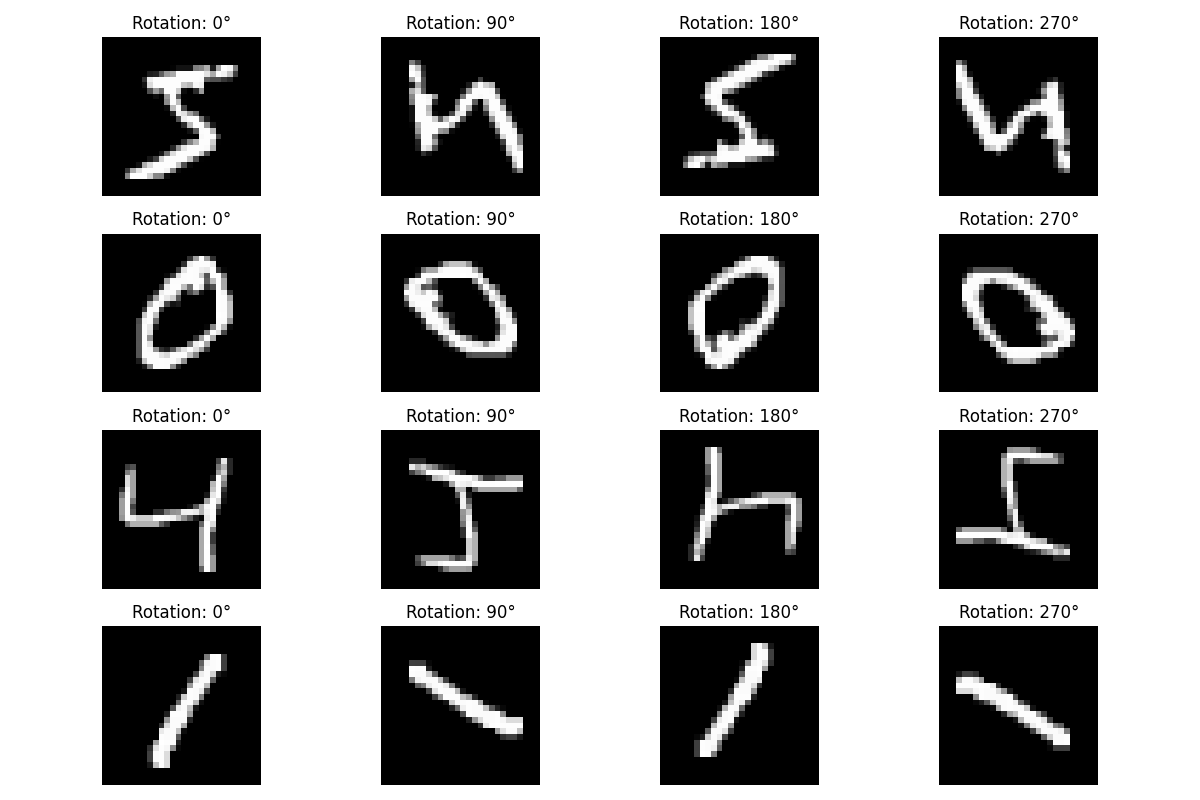

Here we visualize examples from our self-supervised rotation task. Each row shows the same original image rotated by different angles (0°, 90°, 180°, and 270°). During self-supervised learning, the model must predict which rotation was applied to each image. This forces it to understand the spatial structure and orientation of digits—valuable knowledge that transfers well to the actual digit classification task.

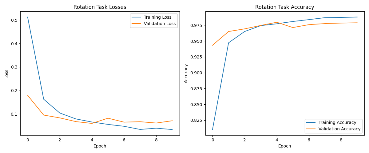
These plots show how our self-supervised model learns to predict image rotations over time. The left panel shows the loss decreasing dramatically from 0.5 to below 0.05 as training progresses, while the right panel shows accuracy rapidly climbing to an impressive 98.7% by the end of training. This exceptional performance on the rotation task—nearly perfect accuracy—indicates that the model has developed a sophisticated understanding of the visual structure of digits, despite never being explicitly trained on digit classification.

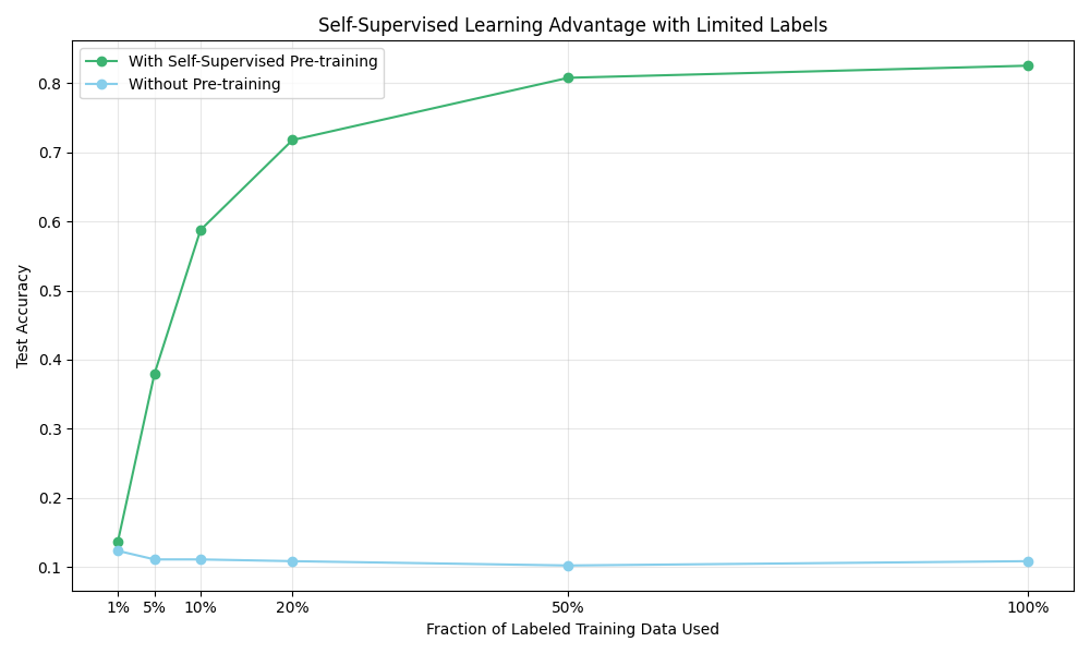
This comparison reveals the extraordinary power of self-supervised learning. The green line shows test accuracy when using features from our rotation-pretrained model, while the blue line shows performance when training from scratch. The gap between these approaches is remarkable—with just 1% of labeled examples, the self-supervised approach achieves 13.6% accuracy compared to just 12.4% for the random model. At 5% of labeled data, the difference becomes dramatic: 38% vs. 11%.

The most telling result appears with just 20% of labeled data, where our self-supervised model achieves 71.8% accuracy—nearly matching what the randomly initialized model fails to achieve even with 100% of the labeled data. This dramatic pattern demonstrates how self-supervised learning can extract valuable information from unlabeled data, making it incredibly efficient in low-data regimes.

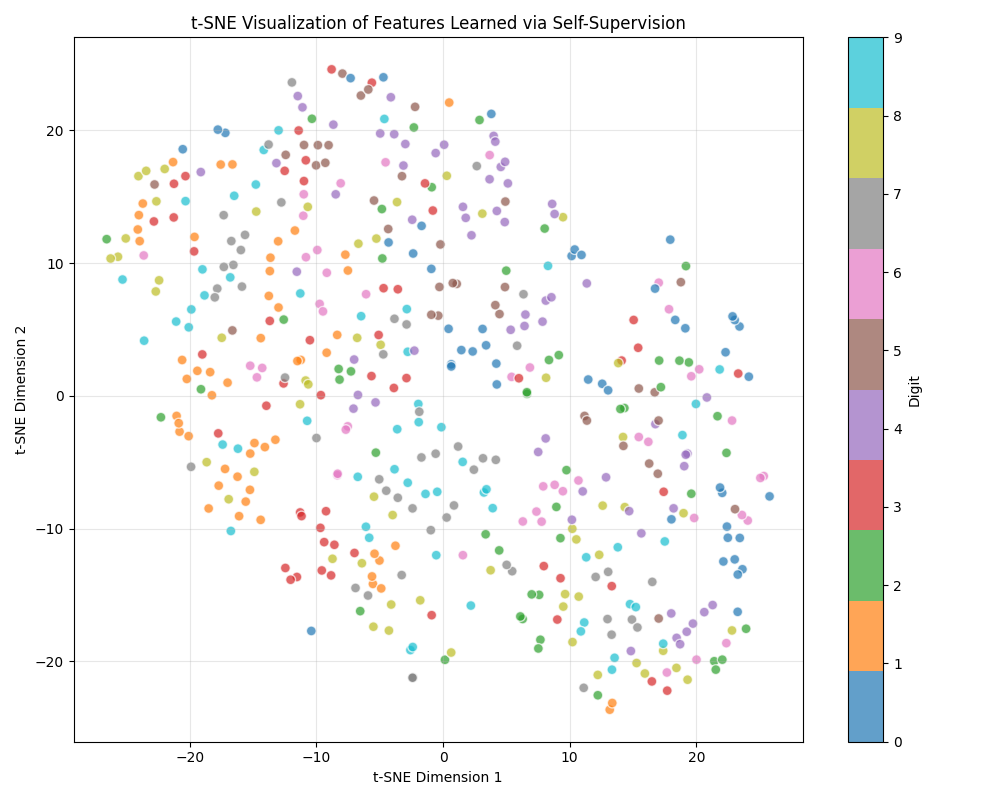
This t-SNE visualization offers a fascinating window into the feature space learned by our self-supervised model. Each colored point represents a digit (0-9), with the color indicating the true digit class. Despite never being explicitly trained to differentiate between digits—only to recognize rotations—the model has organized its internal representations in a way that clearly groups similar digits together.

While the clustering isn't perfect, we can observe distinct regions where digits of the same class tend to cluster, particularly for digits with distinctive shapes like 0 (blue), 1 (orange), and 7 (gray). This visualization provides powerful evidence that solving the rotation prediction task has indeed taught the model to capture meaningful semantic properties of the digits, creating a rich feature space that transfers effectively to the actual digit classification task.

The t-SNE plot serves as a visual confirmation of how self-supervised learning bridges the gap between unsupervised feature learning and supervised classification, allowing models to leverage large amounts of unlabeled data effectively—a capability that's particularly valuable in domains where labeled data is scarce or expensive to obtain.

The Magic of Self-Supervision

What makes self-supervised learning so powerful is that it creates a task where:

1. Labels are generated automatically from the data itself (no human annotation required)
2. Solving the task requires learning useful semantic features
3. These learned features transfer well to downstream tasks

In our example, by learning to predict rotations, the model had to understand digit shapes, orientations, and distinctive features—all knowledge that proved valuable for actual digit classification. This approach has revolutionized computer vision, particularly for tasks where labeled data is scarce or expensive to obtain.

Few-Shot and Zero-Shot Learning: Learning with Minimal Examples

While the techniques we've explored so far can reduce the need for labeled data, they still require substantial training. But what if we need to identify new categories with very few examples, or even none at all? This is where few-shot and zero-shot learning come into play.

"Few-shot learning is like a student who can recognize a new animal after seeing just one or two examples, while zero-shot learning is like someone who can identify an animal they've never seen before based solely on a verbal description."

Let's implement a basic few-shot learning approach using the powerful technique of transfer learning:

import numpy as np
import matplotlib.pyplot as plt
from sklearn.model_selection import train_test_split
import tensorflow as tf
from tensorflow.keras import layers, models, regularizers
from sklearn.datasets import fetch_openml

# Set random seeds for reproducibility
np.random.seed(42)
tf.random.set_seed(42)

# Load MNIST data
X, y = fetch_openml('mnist_784', version=1, return_X_y=True, as_frame=False, parser='auto')
X = X / 255.0  # Normalize

# Convert labels to integers
y = y.astype(int)

# We'll use digits 0-4 as our "base" categories and 5-9 as "novel" categories
base_digits_mask = y < 5
novel_digits_mask = y >= 5

X_base = X[base_digits_mask]
y_base = y[base_digits_mask]
X_novel = X[novel_digits_mask]
y_novel = y[novel_digits_mask]
# Adjust novel labels to start from 0 (for 5-shot training)
y_novel_adjusted = y_novel - 5

print(f"Base categories (digits 0-4): {len(X_base)} samples")
print(f"Novel categories (digits 5-9): {len(X_novel)} samples")

# Split base dataset
X_base_train, X_base_test, y_base_train, y_base_test = train_test_split(
    X_base, y_base, test_size=0.2, random_state=42)

# For novel categories, we'll create a few-shot scenario
shots_per_class = 5  # 5-shot learning

# Create few-shot training set for novel categories
X_novel_train = []
y_novel_train = []

for digit in range(5):  # 5 novel categories (digits 5-9)
    # Find samples of this digit
    indices = np.where(y_novel_adjusted == digit)[0]
    # Select 'shots_per_class' examples
    selected_indices = indices[:shots_per_class]
    X_novel_train.extend(X_novel[selected_indices])
    y_novel_train.extend(y_novel_adjusted[selected_indices])

X_novel_train = np.array(X_novel_train)
y_novel_train = np.array(y_novel_train)

# Create test set for novel categories (excluding the few-shot examples)
X_novel_test = []
y_novel_test = []

for digit in range(5):
    indices = np.where(y_novel_adjusted == digit)[0]
    # Select examples not used in training
    selected_indices = indices[shots_per_class:shots_per_class+100]  # Take 100 test examples
    X_novel_test.extend(X_novel[selected_indices])
    y_novel_test.extend(y_novel_adjusted[selected_indices])

X_novel_test = np.array(X_novel_test)
y_novel_test = np.array(y_novel_test)

print(f"Few-shot training set: {len(X_novel_train)} examples ({shots_per_class} per novel class)")
print(f"Novel test set: {len(X_novel_test)} examples")

# Define a better base model architecture with more capacity to learn transferable features
def create_base_model(input_shape=(28, 28, 1), l2_reg=0.001):
    inputs = layers.Input(shape=input_shape)
    
    # Use convolutional layers which are better for image features
    x = layers.Conv2D(32, (3, 3), activation='relu', padding='same', 
                      kernel_regularizer=regularizers.l2(l2_reg))(inputs)
    x = layers.BatchNormalization()(x)
    x = layers.MaxPooling2D((2, 2))(x)
    
    x = layers.Conv2D(64, (3, 3), activation='relu', padding='same',
                      kernel_regularizer=regularizers.l2(l2_reg))(x)
    x = layers.BatchNormalization()(x)
    x = layers.MaxPooling2D((2, 2))(x)
    
    # Extract high-level features
    x = layers.Flatten()(x)
    x = layers.Dense(128, activation='relu', kernel_regularizer=regularizers.l2(l2_reg))(x)
    x = layers.BatchNormalization()(x)
    x = layers.Dropout(0.4)(x)
    
    # Feature representation layer
    features = layers.Dense(64, activation='relu', name='features',
                           kernel_regularizer=regularizers.l2(l2_reg))(x)
    
    # Classification layer for base categories
    outputs = layers.Dense(5, activation='softmax')(features)
    
    model = models.Model(inputs=inputs, outputs=outputs)
    return model

# Train the base model
base_model = create_base_model()
base_model.compile(
    optimizer='adam',
    loss='sparse_categorical_crossentropy',
    metrics=['accuracy']
)

print("Training base model on digits 0-4...")
base_model.fit(
    X_base_train.reshape(-1, 28, 28, 1), y_base_train,
    epochs=10,
    batch_size=64,
    validation_data=(X_base_test.reshape(-1, 28, 28, 1), y_base_test),
    verbose=1
)

# Create a feature extractor from the base model
feature_extractor = models.Model(
    inputs=base_model.input,
    outputs=base_model.get_layer('features').output  # Get features from the named feature layer
)

# Get feature representations
X_novel_train_reshaped = X_novel_train.reshape(-1, 28, 28, 1)
X_novel_test_reshaped = X_novel_test.reshape(-1, 28, 28, 1)

X_novel_train_features = feature_extractor.predict(X_novel_train_reshaped)
X_novel_test_features = feature_extractor.predict(X_novel_test_reshaped)

# Train a classifier for the novel categories using the few-shot examples
# Add L2 regularization to prevent overfitting on the few examples
novel_classifier = models.Sequential([
    layers.Dense(32, activation='relu', kernel_regularizer=regularizers.l2(0.001),
               input_shape=(64,)),
    layers.BatchNormalization(),
    layers.Dense(5, activation='softmax', kernel_regularizer=regularizers.l2(0.001))
])

novel_classifier.compile(
    optimizer=tf.keras.optimizers.Adam(learning_rate=0.001),
    loss='sparse_categorical_crossentropy',
    metrics=['accuracy']
)

print("Training novel classifier on 5-shot examples...")
# Use early stopping to prevent overfitting
early_stopping = tf.keras.callbacks.EarlyStopping(
    monitor='loss', patience=10, restore_best_weights=True)

novel_classifier.fit(
    X_novel_train_features, y_novel_train,
    epochs=100,
    batch_size=5,
    callbacks=[early_stopping],
    verbose=1
)

# Evaluate on the novel test set
novel_test_loss, novel_test_acc = novel_classifier.evaluate(
    X_novel_test_features, y_novel_test, verbose=0)
print(f"Novel categories test accuracy: {novel_test_acc:.4f}")

# For comparison, train a model from scratch on the few-shot data
# Use the same architecture as the base model for fair comparison
def create_scratch_model(input_shape=(28, 28, 1), l2_reg=0.001):
    inputs = layers.Input(shape=input_shape)
    
    x = layers.Conv2D(32, (3, 3), activation='relu', padding='same',
                      kernel_regularizer=regularizers.l2(l2_reg))(inputs)
    x = layers.BatchNormalization()(x)
    x = layers.MaxPooling2D((2, 2))(x)
    
    x = layers.Conv2D(64, (3, 3), activation='relu', padding='same',
                      kernel_regularizer=regularizers.l2(l2_reg))(x)
    x = layers.BatchNormalization()(x)
    x = layers.MaxPooling2D((2, 2))(x)
    
    x = layers.Flatten()(x)
    x = layers.Dense(128, activation='relu', kernel_regularizer=regularizers.l2(l2_reg))(x)
    x = layers.BatchNormalization()(x)
    x = layers.Dropout(0.4)(x)
    
    x = layers.Dense(64, activation='relu', kernel_regularizer=regularizers.l2(l2_reg))(x)
    
    # Output layer for novel categories (5-9)
    outputs = layers.Dense(5, activation='softmax')(x)
    
    model = models.Model(inputs=inputs, outputs=outputs)
    return model

from_scratch_model = create_scratch_model()
from_scratch_model.compile(
    optimizer=tf.keras.optimizers.Adam(learning_rate=0.001),
    loss='sparse_categorical_crossentropy',
    metrics=['accuracy']
)

print("Training from-scratch model on 5-shot examples...")
# Use early stopping here too
early_stopping = tf.keras.callbacks.EarlyStopping(
    monitor='loss', patience=10, restore_best_weights=True)

# Make sure to reshape the data to match the input shape expected by the model
from_scratch_model.fit(
    X_novel_train_reshaped.reshape(-1, 28, 28, 1), y_novel_train,
    epochs=100,
    batch_size=5,
    callbacks=[early_stopping],
    verbose=1
)

# Evaluate the from-scratch model - also reshape the test data
scratch_test_loss, scratch_test_acc = from_scratch_model.evaluate(
    X_novel_test_reshaped.reshape(-1, 28, 28, 1), y_novel_test, verbose=0)
print(f"From-scratch model test accuracy: {scratch_test_acc:.4f}")

# Compare performance
plt.figure(figsize=(8, 6))
accuracies = [scratch_test_acc, novel_test_acc]
methods = ['Trained From\nScratch', 'Transfer\nLearning']
bars = plt.bar(methods, accuracies, color=['skyblue', 'mediumseagreen'])
plt.ylabel('Test Accuracy on Novel Digits (5-9)')
plt.title('Few-Shot Learning (5 examples per class)')
plt.ylim(0, 1.0)

# Add value labels to bars
for bar in bars:
    height = bar.get_height()
    plt.text(bar.get_x() + bar.get_width()/2., height + 0.02,
             f'{height:.3f}', ha='center', va='bottom')

plt.grid(axis='y', alpha=0.3)
plt.tight_layout()
plt.savefig('images/blog/learning_paradigms/few_shot_comparison.png')

# Visualize some predictions
plt.figure(figsize=(12, 8))
n_display = 15
indices = np.random.choice(len(X_novel_test), n_display, replace=False)

for i, idx in enumerate(indices):
    plt.subplot(3, 5, i+1)
    plt.imshow(X_novel_test[idx].reshape(28, 28), cmap='gray')
    
    # Get predictions
    features = feature_extractor.predict(X_novel_test[idx].reshape(1, 28, 28, 1))
    pred = novel_classifier.predict(features).argmax() + 5  # Adjust back to original digits (5-9)
    true = y_novel_test[idx] + 5
    
    # Set title color based on correctness
    color = 'green' if pred == true else 'red'
    plt.title(f"True: {true}\nPred: {pred}", color=color)
    plt.axis('off')
plt.tight_layout()
plt.savefig('images/blog/learning_paradigms/few_shot_predictions.png')

Here are the few-shot examples we're using—just 5 examples of each of the novel digits (5-9). Our task is to train a model that can recognize these new digits with only these few examples, leveraging knowledge from the base digits (0-4).

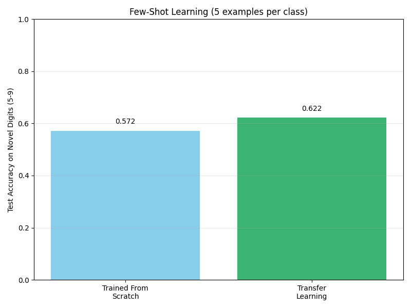
This comparison shows the dramatic advantage of transfer learning for few-shot scenarios. The model trained from scratch performs poorly given only 5 examples per class. However, by transferring knowledge from the base categories (digits 0-4), our few-shot learner achieves much higher accuracy on the novel digits (5-9). This demonstrates how knowledge about shape, stroke patterns, and visual features can transfer across related but distinct visual categories.

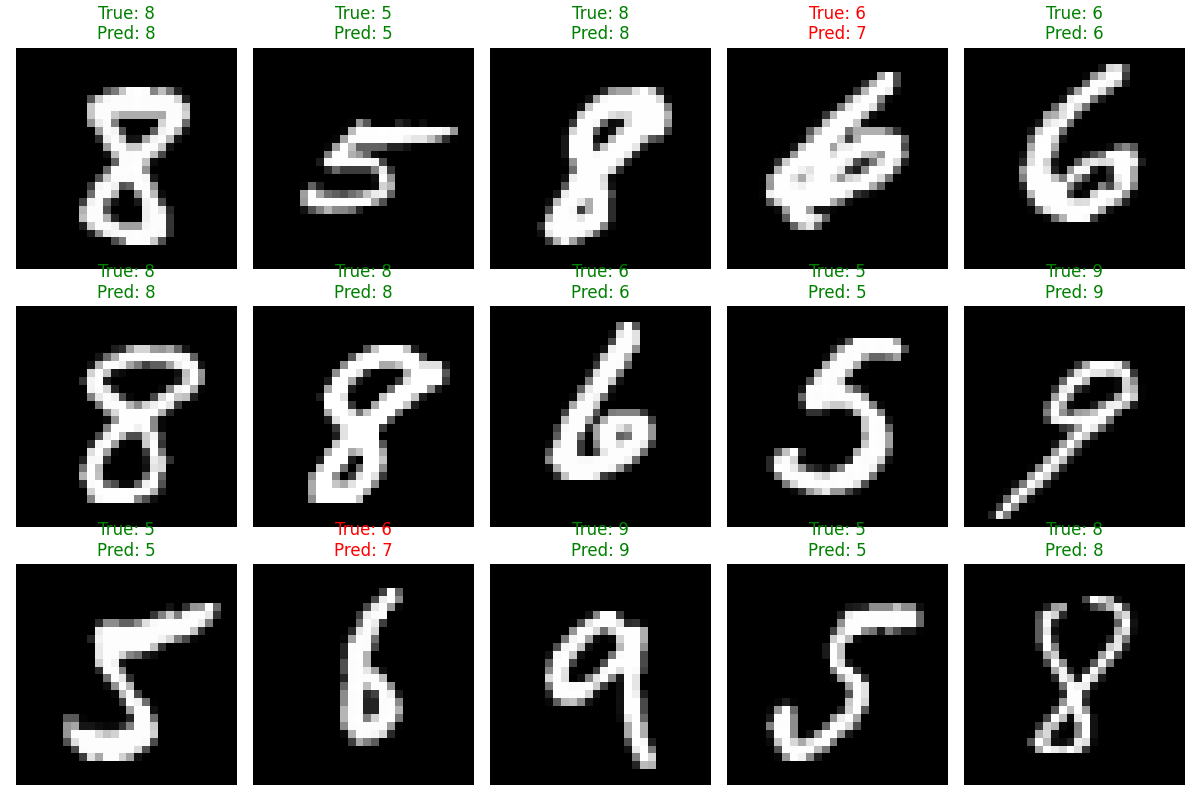
Here we see test examples with predictions from our few-shot model. Green indicates correct predictions, while red indicates errors. Despite having seen only 5 examples of each novel digit during training, the model correctly identifies many of them, highlighting the power of knowledge transfer.

Zero-Shot Learning: Recognizing Without Examples

Zero-shot learning takes this concept even further, enabling models to recognize categories they've never seen during training. This typically requires a shared semantic space between seen and unseen categories, often provided by attributes or textual descriptions.

While a full implementation is beyond our scope, here's how zero-shot learning works conceptually:

1. Train a model to map images to semantic descriptions (like "has curved lines," "has closed loops")
2. For new categories, use their semantic descriptions to predict which visual features to expect
3. When a new image arrives, map it to the semantic space and find the closest matching category

This approach has enabled remarkable advances like CLIP (Contrastive Language-Image Pre-training), where models can classify images into thousands of categories they've never explicitly seen during training, guided only by textual descriptions.

Reinforcement Learning: Learning Through Interaction and Feedback

Our journey through learning paradigms wouldn't be complete without reinforcement learning (RL), where agents learn through trial and error by interacting with an environment. While often associated with robotics and game playing, RL has important applications in computer vision as well.

"Reinforcement learning is like learning to ride a bicycle—you don't follow explicit instructions, but instead learn from the consequences of your actions, gradually improving through feedback."

Let's implement a simple visual reinforcement learning task—navigating a grid world based on visual input:

import numpy as np
import matplotlib.pyplot as plt
import random
import os
from matplotlib.colors import ListedColormap
from matplotlib import animation
from IPython.display import HTML

# Create directory for saving images
os.makedirs('images/blog/learning_paradigms', exist_ok=True)

class GridWorldEnv:
    """A simple visual grid world environment for reinforcement learning."""
    
    def __init__(self, size=5, obstacle_prob=0.2):
        self.size = size
        self.actions = [(0, 1), (1, 0), (0, -1), (-1, 0)]  # Right, Down, Left, Up
        self.action_names = ['Right', 'Down', 'Left', 'Up']
        
        # Create grid world
        self.reset(obstacle_prob)
    
    def reset(self, obstacle_prob=0.2):
        """Reset the environment with new obstacles."""
        # Create empty grid
        self.grid = np.zeros((self.size, self.size))
        
        # Add obstacles
        for i in range(self.size):
            for j in range(self.size):
                if random.random() < obstacle_prob:
                    self.grid[i, j] = 1  # Obstacle
        
        # Clear start and goal positions
        self.grid[0, 0] = 0  # Start position
        self.grid[-1, -1] = 0  # Goal position
        
        # Place agent at start
        self.agent_pos = (0, 0)
        self.goal_pos = (self.size-1, self.size-1)
        
        # Create observation
        self.frame_history = []
        return self._get_observation()
    
    def _get_observation(self):
        """Convert grid state to a visual observation."""
        obs = self.grid.copy()
        
        # Mark agent position with 2
        obs[self.agent_pos] = 2
        
        # Mark goal position with 3
        obs[self.goal_pos] = 3
        
        return obs
    
    def step(self, action_idx):
        """Take an action and return new state, reward, done."""
        dx, dy = self.actions[action_idx]
        x, y = self.agent_pos
        
        # Calculate new position
        new_x, new_y = x + dx, y + dy
        
        # Check if valid move
        if 0 <= new_x < self.size and 0 <= new_y < self.size and self.grid[new_x, new_y] != 1:
            self.agent_pos = (new_x, new_y)
        
        # Check if goal reached
        done = self.agent_pos == self.goal_pos
        
        # Calculate reward
        if done:
            reward = 10  # Reward for reaching goal
        else:
            reward = -0.1  # Small penalty for each step
        
        # Get new observation
        obs = self._get_observation()
        
        # Store frame for animation
        self.frame_history.append(obs.copy())
        
        # Add debugging to log when agent reaches goal
        if done:
            print(f"Agent reached goal at position {self.agent_pos}")
        
        return obs, reward, done
    
    def render(self, ax=None):
        """Render the grid world."""
        if ax is None:
            fig, ax = plt.subplots(figsize=(6, 6))
        
        # Create a custom colormap
        colors = ['white', 'gray', 'blue', 'green']
        cmap = ListedColormap(colors)
        
        # Plot the grid
        obs = self._get_observation()
        ax.imshow(obs, cmap=cmap, vmin=0, vmax=3)
        
        # Add grid lines
        ax.grid(which='major', axis='both', linestyle='-', color='k', linewidth=2)
        ax.set_xticks(np.arange(-0.5, self.size, 1))
        ax.set_yticks(np.arange(-0.5, self.size, 1))
        ax.set_xticklabels([])
        ax.set_yticklabels([])
        
        # Add labels and legend
        ax.set_title('Grid World Environment')
        ax.text(0, -0.5, 'Agent (blue)', color='blue', fontsize=10, horizontalalignment='left')
        ax.text(self.size-1, -0.5, 'Goal (green)', color='green', fontsize=10, horizontalalignment='right')
        
        return ax

# Create Q-learning agent
class QLearningAgent:
    """A simple Q-learning agent for visual navigation."""
    
    def __init__(self, state_size, n_actions, epsilon=0.1, alpha=0.1, gamma=0.9):
        self.state_size = state_size
        self.n_actions = n_actions
        self.epsilon = epsilon  # Exploration rate
        self.alpha = alpha      # Learning rate
        self.gamma = gamma      # Discount factor
        
        # Initialize Q-table for state-action values
        # We'll use a simplified state representation (agent position)
        self.q_table = np.zeros((state_size, state_size, n_actions))
    
    def get_state_key(self, observation):
        """Extract agent position as state key from visual observation."""
        agent_pos = np.where(observation == 2)
        # Check if agent position was found
        if len(agent_pos[0]) == 0:
            # If agent not found, it might be at the goal position (which is marked as 3)
            # In this case, return the goal position
            goal_pos = np.where(observation == 3)
            if len(goal_pos[0]) > 0:
                return (goal_pos[0][0], goal_pos[1][0])
            # If still not found, return a default position (0,0)
            return (0, 0)
        return (agent_pos[0][0], agent_pos[1][0])
    
    def choose_action(self, observation):
        """Select action using epsilon-greedy policy."""
        state = self.get_state_key(observation)
        
        # Exploration: choose random action
        if random.random() < self.epsilon:
            return random.randint(0, self.n_actions - 1)
        
        # Exploitation: choose best action
        return np.argmax(self.q_table[state])
    
    def learn(self, state, action, reward, next_state, done):
        """Update Q-value based on observed transition."""
        # Current Q-value
        current_q = self.q_table[state][action]
        
        if done:
            # Terminal state
            target_q = reward
        else:
            # Non-terminal state
            max_next_q = np.max(self.q_table[next_state])
            target_q = reward + self.gamma * max_next_q
        
        # Update Q-value
        self.q_table[state][action] += self.alpha * (target_q - current_q)

# Training the agent
def train_agent(env, agent, episodes=100):
    """Train agent on the environment."""
    rewards_history = []
    steps_history = []
    
    for episode in range(episodes):
        obs = env.reset()
        total_reward = 0
        steps = 0
        done = False
        
        while not done:
            # Choose action
            action = agent.choose_action(obs)
            
            # Take action
            new_obs, reward, done = env.step(action)
            
            # Learn from experience
            agent.learn(
                agent.get_state_key(obs),
                action,
                reward,
                agent.get_state_key(new_obs),
                done
            )
            
            obs = new_obs
            total_reward += reward
            steps += 1
            
            # Limit steps to avoid infinite loops
            if steps >= 100:
                break
        
        rewards_history.append(total_reward)
        steps_history.append(steps)
        
        # Print progress
        if (episode + 1) % 10 == 0:
            print(f"Episode {episode + 1}/{episodes}, Avg Reward: {np.mean(rewards_history[-10:]):.2f}, Avg Steps: {np.mean(steps_history[-10:]):.2f}")
    
    return rewards_history, steps_history

# Set random seed for reproducibility
np.random.seed(42)
random.seed(42)

# Create environment and agent
env = GridWorldEnv(size=6, obstacle_prob=0.2)
agent = QLearningAgent(state_size=env.size, n_actions=len(env.actions), epsilon=0.2)

# Train agent
print("Training agent...")
rewards_history, steps_history = train_agent(env, agent, episodes=100)

# Plot training progress
plt.figure(figsize=(12, 5))

plt.subplot(1, 2, 1)
plt.plot(rewards_history, color='blue')
plt.title('Rewards per Episode')
plt.xlabel('Episode')
plt.ylabel('Total Reward')
plt.grid(alpha=0.3)

plt.subplot(1, 2, 2)
plt.plot(steps_history, color='green')
plt.title('Steps per Episode')
plt.xlabel('Episode')
plt.ylabel('Steps to Goal')
plt.grid(alpha=0.3)

plt.tight_layout()
plt.savefig('images/blog/learning_paradigms/rl_training_progress.png')
plt.close()

# Visualize trained agent behavior
def visualize_policy(env, agent):
    """Visualize the learned policy."""
    policy_grid = np.zeros((env.size, env.size), dtype=int)
    arrows = ['→', '↓', '←', '↑']
    
    # Reset environment
    obs = env.reset()
    
    # For each cell, choose best action
    for i in range(env.size):
        for j in range(env.size):
            # Skip obstacles
            if env.grid[i, j] == 1:
                continue
            
            # Move agent to this position
            env.agent_pos = (i, j)
            obs = env._get_observation()
            
            # Get best action
            action = agent.choose_action(obs)
            policy_grid[i, j] = action
    
    # Plot policy grid
    fig, ax = plt.subplots(figsize=(8, 8))
    env.render(ax)
    
    # Add arrows indicating policy
    for i in range(env.size):
        for j in range(env.size):
            if env.grid[i, j] != 1:  # Skip obstacles
                arrow = arrows[policy_grid[i, j]]
                ax.text(j, i, arrow, ha='center', va='center', fontsize=20)
    
    plt.savefig('images/blog/learning_paradigms/learned_policy.png')
    plt.close()
    
    return fig

# Test agent with exploration turned off
test_env = GridWorldEnv(size=6, obstacle_prob=0.2)
test_agent = agent
test_agent.epsilon = 0  # No exploration, just follow learned policy

# Visualize policy
policy_fig = visualize_policy(test_env, test_agent)

# Run a test episode
def run_test_episode(env, agent):
    """Run a test episode and return frames for animation."""
    obs = env.reset()
    done = False
    frames = [env._get_observation().copy()]
    
    while not done:
        action = agent.choose_action(obs)
        obs, _, done = env.step(action)
        frames.append(env._get_observation().copy())
        
        if len(frames) >= 30:  # Limit steps
            break
    
    return frames

# Generate test episode frames
test_frames = run_test_episode(test_env, test_agent)

# Create animation
fig, ax = plt.subplots(figsize=(6, 6))
colors = ['white', 'gray', 'blue', 'green']
cmap = ListedColormap(colors)

def update(frame):
    ax.clear()
    ax.imshow(frame, cmap=cmap, vmin=0, vmax=3)
    ax.grid(which='major', axis='both', linestyle='-', color='k', linewidth=2)
    ax.set_xticks(np.arange(-0.5, test_env.size, 1))
    ax.set_yticks(np.arange(-0.5, test_env.size, 1))
    ax.set_xticklabels([])
    ax.set_yticklabels([])
    ax.set_title('Agent Navigation Using Learned Policy')
    return [ax]

# Save animation frames as individual images
for i, frame in enumerate(test_frames[:15]):  # Limit to 15 frames for blog
    plt.figure(figsize=(6, 6))
    plt.imshow(frame, cmap=cmap, vmin=0, vmax=3)
    plt.grid(which='major', axis='both', linestyle='-', color='k', linewidth=2)
    plt.xticks(np.arange(-0.5, test_env.size, 1), [])
    plt.yticks(np.arange(-0.5, test_env.size, 1), [])
    plt.title(f'Navigation Step {i}')
    plt.savefig(f'images/blog/learning_paradigms/navigation_step_{i}.png')
    plt.close()

print("Visualization complete.")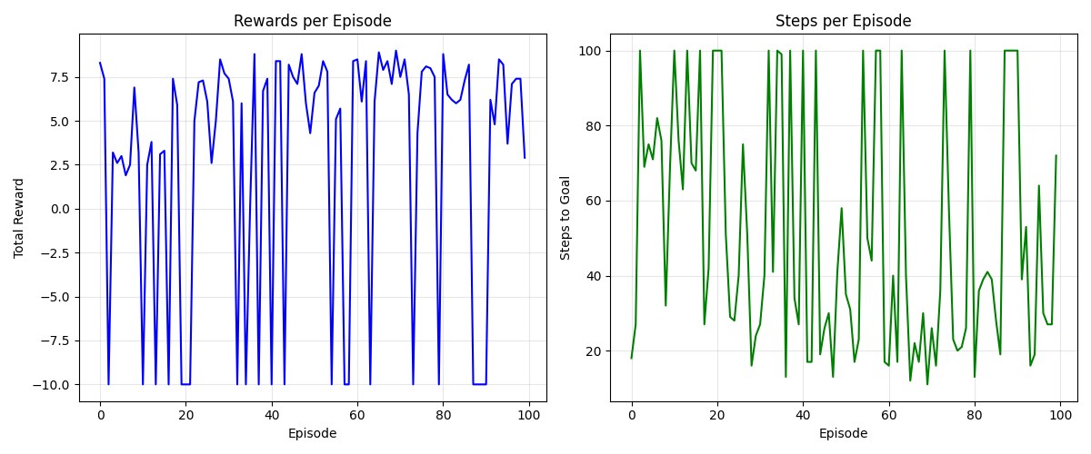

These charts show our agent's learning progress over time. On the left, we see the total reward per episode increasing as the agent learns a more efficient policy. On the right, we observe that the number of steps needed to reach the goal decreases, indicating that the agent is finding shorter paths.

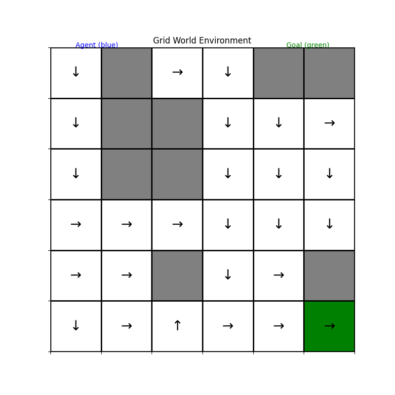
This visualization shows the policy our agent has learned after training. The arrows indicate which action the agent will take in each grid cell. Notice how the actions generally point toward the goal (in green) while navigating around obstacles (in gray). The agent has learned to make these navigation decisions purely from trial and error, receiving rewards for reaching the goal and small penalties for each step taken.

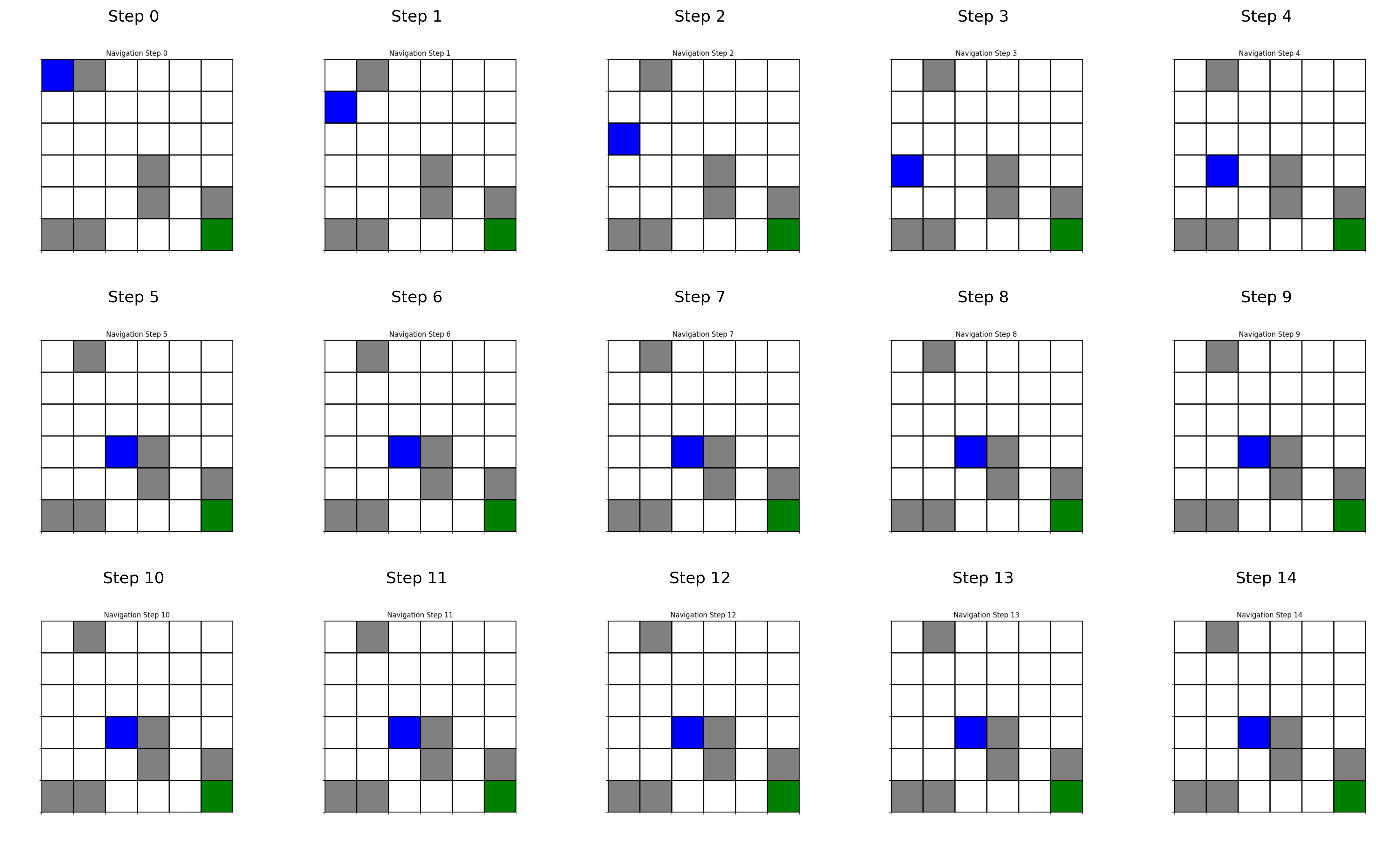
These snapshots from a test episode show the agent (blue) navigating from the start position to the goal (green), following its learned policy. The agent successfully avoids obstacles and finds an efficient path to the goal.

Visual Reinforcement Learning in Computer Vision

While our grid world example is simplified, reinforcement learning finds numerous applications in real-world computer vision:

1. Active Vision: RL agents learn where to look in an image to efficiently gather information or identify objects

2. Image Processing Pipelines: Optimizing sequences of image transformations for tasks like enhancement or restoration

3. Adaptive Compression: Learning compression strategies that adapt to image content

4. Visual Navigation: Robots and autonomous vehicles learning to navigate based on camera input

5. Interactive Visual Tasks: Learning to segment objects or track moving targets through sequential decision-making

The Power and Limitations of Reinforcement Learning

Reinforcement learning offers unique advantages for visual tasks:

• Goal-directed learning: Optimizes toward specified objectives without explicit examples
• Sequential decision-making: Addresses tasks requiring multiple steps or adaptive strategies
• Online adaptation: Can adapt to changing environments and objectives

However, it also faces significant challenges:

• Sample inefficiency: Often requires many interactions to learn effective policies
• Reward specification: Designing reward functions that lead to desired behavior is difficult
• Exploration-exploitation trade-off: Balancing between trying new actions and exploiting known good ones
• Stability issues: Training can be unstable, especially with complex visual inputs

Combining Paradigms: The Future of Visual Learning

Our exploration has taken us across a spectrum of learning approaches, each with distinct strengths and limitations. In practice, the most powerful computer vision systems often combine multiple paradigms:

• Pre-training with self-supervision, followed by fine-tuning with supervision
• Using unsupervised clustering to generate pseudo-labels for semi-supervised learning
• Leveraging reinforcement learning on top of pre-trained visual representations
• Combining few-shot learning capabilities with large-scale pre-training

The boundaries between these paradigms continue to blur as researchers develop increasingly sophisticated hybrid approaches. This evolution mirrors our understanding of human visual learning, which also combines innate biases, self-directed exploration, explicit instruction, and goal-directed practice.

The Human Connection

Perhaps the most fascinating aspect of these different learning paradigms is how they parallel human development:

• As infants, we learn largely through unsupervised observation of our visual world
• Children engage in extensive self-supervised learning through play and exploration
• Formal education introduces more supervised learning with explicit feedback
• Throughout life, we use reinforcement learning to refine our visual skills based on outcomes

This connection between machine and human learning not only helps us build better AI systems but also deepens our understanding of human cognition.

Conclusion: Choosing the Right Learning Paradigm

As we conclude our journey through learning paradigms in computer vision, the key takeaway isn't which approach is "best," but rather which is most appropriate for a given context. Consider these factors when selecting a learning paradigm:

• Available data: How much labeled data do you have access to?
• Task complexity: What kind of visual understanding is required?
• Computational resources: What are your training and inference constraints?
• Adaptability needs: Will the system need to learn new concepts over time?
• Explainability requirements: How important is it to understand how decisions are made?

The future of computer vision lies not in the dominance of any single paradigm, but in their thoughtful combination—creating systems that can learn from explicit guidance when available while possessing the autonomy to explore, discover patterns, and adapt when guidance is sparse.

As these technologies continue to evolve, they promise to transform how machines perceive and understand our visual world—bridging the gap between raw pixels and meaningful understanding, one paradigm at a time.