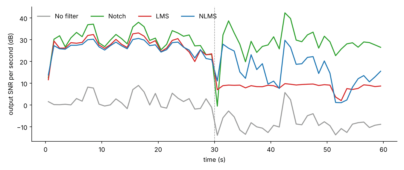
An ECG measures millivolts on the skin. The mains wiring in the room radiates at 50 or 60 Hz, and the body picks it up like an antenna. The result is a hum on top of the heartbeat, often larger than the heartbeat itself.
One classic fix is adaptive noise cancellation. Put a second sensor where it picks up the hum but not the heart (the reference), and let a filter learn how the hum in the reference relates to the hum on the ECG electrode. Then subtract the prediction. The two textbook algorithms for "let a filter learn" are LMS and NLMS.
This article runs both on a real recording and asks three questions:
- How well does each one clean the signal?
- What happens when the interference suddenly gets louder?
- Is an adaptive filter worth it here, compared to a fixed notch filter?
All the numbers below come from one script that you can run yourself: notebook-code/lms-vs-nlms.
The setup
The signal. 60 seconds of a real ECG: record 208 of the MIT-BIH Arrhythmia Database, sampled at 360 Hz, as shipped with SciPy (scipy.datasets.electrocardiogram).
The interference. I add it myself, so the clean signal is known and the result can be measured exactly:
- 60 Hz plus its third harmonic (180 Hz), with a phase that drifts slowly at random, as real mains does.
- For the first 30 seconds its amplitude is 0.5 mV. At t = 30 s it jumps to 2.0 mV, as if a motor or a charger had been switched on nearby. That is four times the amplitude, sixteen times the power.
The reference. The same source as the reference sensor would see it: a different gain (×1.7), a different phase, a little sensor noise, and no ECG at all.
fs = 360
ecg = datasets.electrocardiogram()[: 60 * fs]
t = np.arange(ecg.size) / fs

phase = np.cumsum(rng.normal(0, 0.002, ecg.size))          # slow random phase drift
amp = np.where(t < 30, 0.5, 2.0)                            # x4 at t = 30 s
mains = amp * (np.sin(2*np.pi*60*t + phase) + 0.3*np.sin(2*np.pi*180*t + 3*phase))
primary = ecg + mains                                       # what the ECG electrode records

ref = 1.7 * amp * (np.sin(2*np.pi*60*t + phase + 0.9) + 0.3*np.sin(2*np.pi*180*t + 3*phase + 2.1))
ref += rng.normal(0, 0.01, ecg.size)
The measure. Signal-to-noise ratio (SNR): the power of the clean ECG divided by the power of whatever is left that is not the ECG, in decibels. Higher is better; +10 dB means the leftover noise is ten times smaller.
Before any filtering, the SNR is 3.4 dB in the first half and −4.9 dB in the second half. Negative means the hum is stronger than the heartbeat.
The two algorithms
Both use the same filter: an FIR filter with 8 taps. It takes the last 8 samples of the reference, , and predicts the hum on the ECG electrode as . The cleaned output is the error, , where is the recorded signal.
The trick is that the filter can only predict the part of that is related to the reference, which is the hum. So making as small as possible removes the hum and leaves the heartbeat.
LMS (least mean squares) nudges the weights against the error after every sample:
NLMS (normalized LMS) does the same, but divides the step by the current power of the reference:
That one division is the whole difference. In LMS, the effective step grows with the input power: if the reference gets 16 times stronger, every step is 16 times bigger. In NLMS it does not.
def lms(x, d, M, mu, normalized=False, eps=1e-6):
    w, buf, e = np.zeros(M), np.zeros(M), np.empty_like(d)
    for n in range(d.size):
        buf = np.roll(buf, 1); buf[0] = x[n]
        e[n] = d[n] - w @ buf
        step = mu / (eps + buf @ buf) if normalized else mu
        w = w + step * e[n] * buf
    return e
Choosing the step size, honestly
Both algorithms have one knob, the step size . Too small and the filter learns slowly; too large and it overshoots, or diverges.
To keep the comparison fair, I picked each algorithm's best using only the first 30 seconds. That is all an engineer tuning the device would have seen before the interference changed. Then I let both run through the jump.
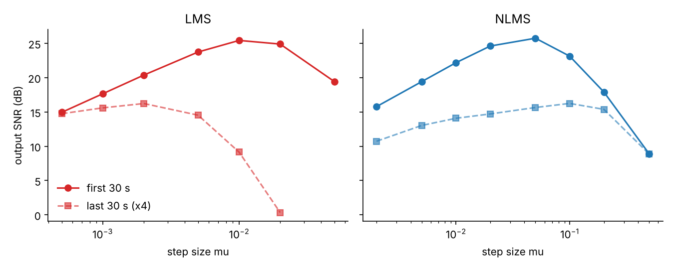
The left panel is the core of the story:
- Before the jump, LMS works best at (25.4 dB).
- After the jump, the same gives only 9.1 dB. The best value has moved five times lower, to 0.002, because the input power rose sixteen times.
- Larger steps are worse: drops to 0.3 dB after the jump, and diverges (the weights blow up to infinity), so it has no point on the dashed line.
NLMS (right panel) has the same shape before the jump, and after it the curve changes much less: every step size from 0.005 to 0.2 stays between 13 and 16.3 dB. Its best value barely moves (0.05 before, 0.1 after).
What happens at t = 30 s
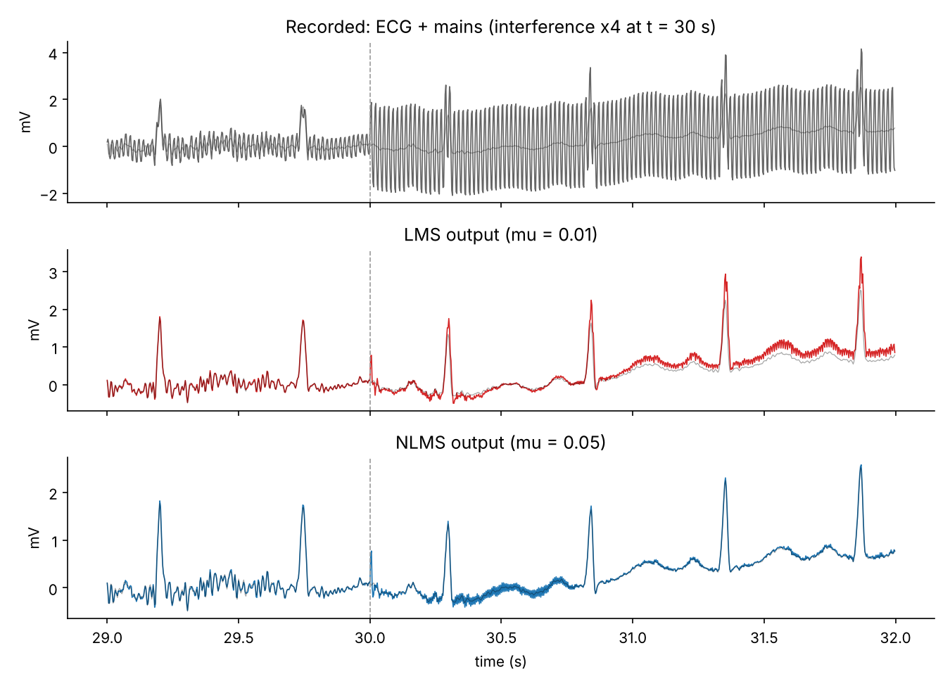
With each algorithm on its tuned step size (LMS 0.01, NLMS 0.05):
| SNR, first 30 s | SNR, last 30 s | Improvement, last 30 s | |
|---|---|---|---|
| No filter | 3.4 dB | −4.9 dB | |
| LMS ( = 0.01) | 25.4 dB | 9.1 dB | 14.0 dB |
| NLMS ( = 0.05) | 25.8 dB | 15.7 dB | 20.5 dB |
| Notch filters (60 and 180 Hz) | 27.1 dB | 22.9 dB | 27.8 dB |
Before the jump, the two adaptive filters are practically equal: 25.4 dB against 25.8 dB. After it, LMS's step is effectively sixteen times larger than the one it was tuned for, and the output in the figure drifts away from the clean ECG. NLMS keeps the heartbeat shape and ends 6.5 dB ahead.
The one-second SNR over the whole minute shows the same thing:
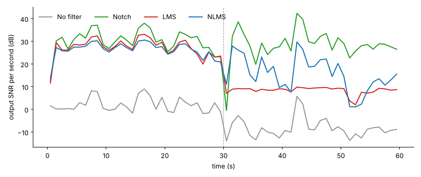
NLMS is not perfect after the jump either. Its SNR moves around much more than before, and it dips to about 1 dB near t = 52 s. The likely reason is simple: the filter always lags the drifting phase a little. With the hum four times larger, the same lag leaves four times more residue.
The uncomfortable result: the notch filter wins
The green line in the last figure is not adaptive at all. It is two fixed notch filters, at 60 Hz and 180 Hz (scipy.signal.iirnotch, quality factor 30), run causally as a real-time device would. It beats both adaptive filters in both halves.
That makes sense once you look at what the problem actually is. The mains frequency is known and stable. A notch filter removes a narrow band around it no matter how loud the hum gets, so the jump does not bother it.
The notch has a cost: it also removes the ECG's own content near 60 and 180 Hz. Measured on the clean ECG alone, the notch output differs from the input by 34.3 dB SNR. That is a small distortion, but not zero.
So when is adaptive cancellation worth it? When you don't know the interference's frequency, or it has no single frequency at all, but you can still measure a reference of it. Classic examples:
- removing the mother's heartbeat from a fetal ECG,
- cancelling engine noise in a headset,
- echo cancellation in phone calls.
Mains hum, with a known and stable frequency, is the textbook example for explaining adaptive noise cancellation, but not the case where it wins.
What this experiment does not show
- The interference is synthetic. The ECG is real, but I generated the hum, its phase drift, and the reference sensor, with parameters I chose. A real reference electrode would be noisier and less perfectly correlated with the hum.
- One recording, one random seed. The exact decibels would change with another patient or another drift pattern. The direction of the result (LMS's best step moves with input power, NLMS's does not) is what the algebra predicts and what the sweep shows.
- Only 8 taps and two algorithms. RLS, or a filter that adapts its own step size, would track faster, at a higher computational cost.
- The "clean" ECG is not perfectly clean. Record 208 already contains some muscle noise, and every SNR here treats that noise as part of the signal.
Takeaways
- LMS's step size is tuned for one input power. If the reference gets 16 times stronger, the effective step gets 16 times larger, and a well-tuned filter becomes a badly tuned one. Here LMS removed 14.0 dB of noise after the jump, against 20.5 dB for NLMS.
- NLMS fixes exactly that, with one division per sample. If the input level can change, use NLMS.
- Check the simple baseline first. For interference at a known, stable frequency, a fixed notch filter was better than both, and needed no reference sensor at all.
Run it yourself
git clone https://github.com/Ahmad-Nayfeh/portfolio-website
cd portfolio-website/notebook-code/lms-vs-nlms
pip install numpy scipy matplotlib pooch
python experiment.py      # about 10 seconds on a laptop CPU
It writes the three figures and a results.json with every number quoted above.
Sources
- B. Widrow et al., "Adaptive noise cancelling: Principles and applications," Proceedings of the IEEE, 63(12), 1975: the original description of the reference-input setup used here.
- S. Haykin, Adaptive Filter Theory, 5th ed., Pearson, 2014: LMS and NLMS derivations and stability.
- G. B. Moody and R. G. Mark, "The impact of the MIT-BIH Arrhythmia Database," IEEE Engineering in Medicine and Biology, 20(3), 2001: the source of the ECG recording.