A damaged ball bearing announces itself in its vibration: every time a ball rolls over a crack, it strikes, and the strikes repeat at a rate set by the bearing's geometry and the shaft speed. Detecting faults from an accelerometer is one of the oldest uses of signal processing in industry, and one of the most popular deep learning benchmarks.
The two usual approaches:
- Engineered features: take the spectrum of the vibration (FFT), summarize it, and train a simple classifier on it.
- A 1D convolutional neural network (CNN) that reads the raw signal and learns its own features.
On the standard dataset, both are reported near 100%. So this article asks the two questions that matter in a plant: what if you have very little labelled data, and what if the signal is noisy?
The full script is in notebook-code/bearing-fft-vs-cnn. Every number below is from one run of it, about 90 seconds on a laptop CPU.
The data
The Case Western Reserve University (CWRU) bearing dataset: an accelerometer on the drive end of a motor, sampled at 12 kHz. Four classes:
- normal,
- a 0.007-inch fault on the inner race,
- the same fault on a ball,
- the same fault on the outer race.
Each class was recorded at four motor loads (0 to 3 horsepower).
Training uses the 0 and 1 HP recordings; testing uses 2 and 3 HP, which the models never see. Every recording is cut into windows of 2,048 samples (0.17 s) with 50% overlap. That gives 940 test windows, about 235 per class.
The split by load matters. Splitting windows at random would put overlapping pieces of the same recording in both training and test, and inflate the score.
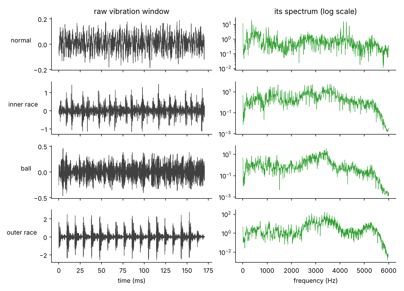
The time signals already show the story: the outer-race fault strikes in a clean, regular rhythm; the inner-race fault less so; the ball fault is buried in the rest of the vibration.
A trap in the data, before anything else
The normal recordings are sampled at 48 kHz, not 12 kHz like the fault recordings. CWRU publishes them together, and it is easy to miss. I checked it by finding the same mechanical peaks (148, 162 and 192 Hz) in both files: they line up only when the normal file is read at 48 kHz.
Mixing the two rates teaches a model to recognize the sampling rate instead of the fault, so the script resamples the normal files to 12 kHz first:
if num in FILES["normal"]:
    x = resample_poly(x, 1, 4)        # 48 kHz -> 12 kHz
That fix turned out not to be enough. More on that below.
The two methods
A. FFT band energies + logistic regression. For each window: apply a Hann window, take the magnitude spectrum up to 6 kHz, average it into 64 bands of about 94 Hz each, and take the log. A logistic regression (a linear classifier) learns from those 64 numbers.
def fft_features(X, bands=64):
    spec = np.abs(np.fft.rfft(X * HANN, axis=1))[:, 1:1025]       # 0-6 kHz
    return np.log1p(spec.reshape(len(X), bands, -1).mean(axis=2))
B. A small 1D CNN on the raw window. It has four convolution blocks; the first uses a wide kernel (64 samples) with a stride of 8, a common design for vibration data (WDCNN). That is 21,780 parameters, trained for 400 steps with Adam.
Both are trained on clean signals. At test time, white noise is added at a chosen signal-to-noise ratio: 10 dB (noise power one tenth of the signal), 5 dB, 0 dB (equal power) and −5 dB (noise three times stronger than the signal).
Training sets are drawn at random with 4, 8, 16, 32, 64 or 160 windows per class. 160 is about all the normal windows the two training loads have. Small sizes are repeated with 5 random draws, larger ones with 3.
Result 1: on clean signals, there is nothing to compare
Both methods reach 100% on the unseen loads, at every training size, even with 4 windows per class. (The single exception is the CNN on the 0–4 kHz input with 4 windows: 99.7%.)
That says more about the dataset than about the methods. These faults were machined into the bearings by electro-discharge, and each one makes a strong, distinctive signature. CWRU is a good teaching dataset and a poor benchmark: anything sensible scores 100% on it.
Result 2: add noise, and the FFT model collapses
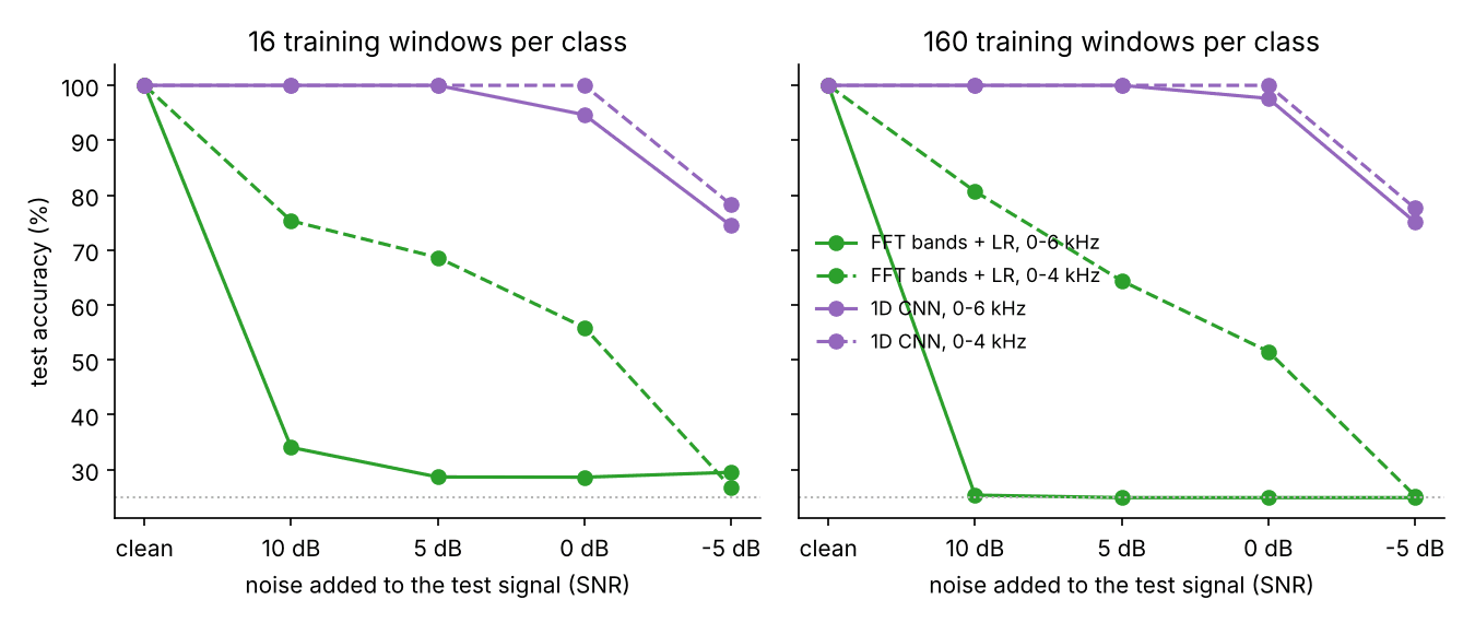
At 10 dB of test noise, which is mild, the FFT model drops from 100% to 25.4%: exactly chance for four classes. Its predictions show why: it calls almost every window "normal" (938 of 940).
The CNN, trained on the same clean windows, keeps 100% at 10 dB and 5 dB, and 97.6% at 0 dB.
Why: the model learned the recording equipment
Look again at the spectra above. The normal one stays high all the way to 6 kHz. The three fault spectra drop steeply above about 5.5 kHz.
That drop is not physics. The 12 kHz fault recordings passed through the recording system's anti-aliasing filter. The normal recordings were made at 48 kHz, and resampling them leaves energy right up to 6 kHz. Measured on the test windows:
| Class | Share of energy above 5.5 kHz (median) |
|---|---|
| normal | 0.23% |
| inner race | 0.0015% |
| outer race | 0.014% |
| ball | 0.0004% |
The normal windows carry 16 to 554 times more of their energy in that band than the fault classes. A linear model finds this immediately; it is the easiest way to separate "normal" from everything else.
White noise has equal power at every frequency, so it fills that band in every window. To a model that learned "energy near 6 kHz means normal", every noisy window looks normal.
The fix: use only 0–4 kHz. For the FFT model, that means using only the spectrum up to 3.75 kHz, averaged into 64 narrower bands. For the CNN, the input is low-pass filtered at 4 kHz, in training and in testing. The dashed lines below are these versions.
The fair comparison
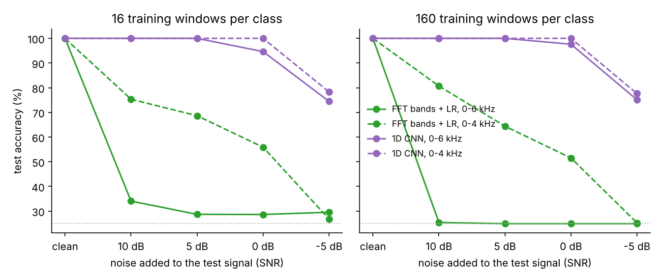
| Test noise | FFT + LR, 0–4 kHz | 1D CNN, 0–4 kHz |
|---|---|---|
| clean | 100% | 100% |
| 10 dB | 80.7% | 100% |
| 5 dB | 64.4% | 100% |
| 0 dB | 51.5% | 100% |
| −5 dB | 25.2% | 77.6% |
160 training windows per class; averages of 3 runs.
Without the giveaway band, the FFT model behaves sensibly, but it degrades steadily. In one of the runs at 0 dB it still gets every normal and inner-race window right, and none of the ball or outer-race windows: it calls almost all of them "inner race".
The CNN loses almost nothing until −5 dB. There, it still recognizes normal, inner race and outer race perfectly, but gets only 10% of the ball faults right. That matches the waveforms above: the ball fault has the weakest, least regular strikes, so it is the first to sink under noise.
Note that low-pass filtering also removes a third of the added white noise (everything between 4 and 6 kHz). So the 0–4 kHz versions face a slightly easier test than the 0–6 kHz ones. That advantage is the same for both methods.
And with less data?
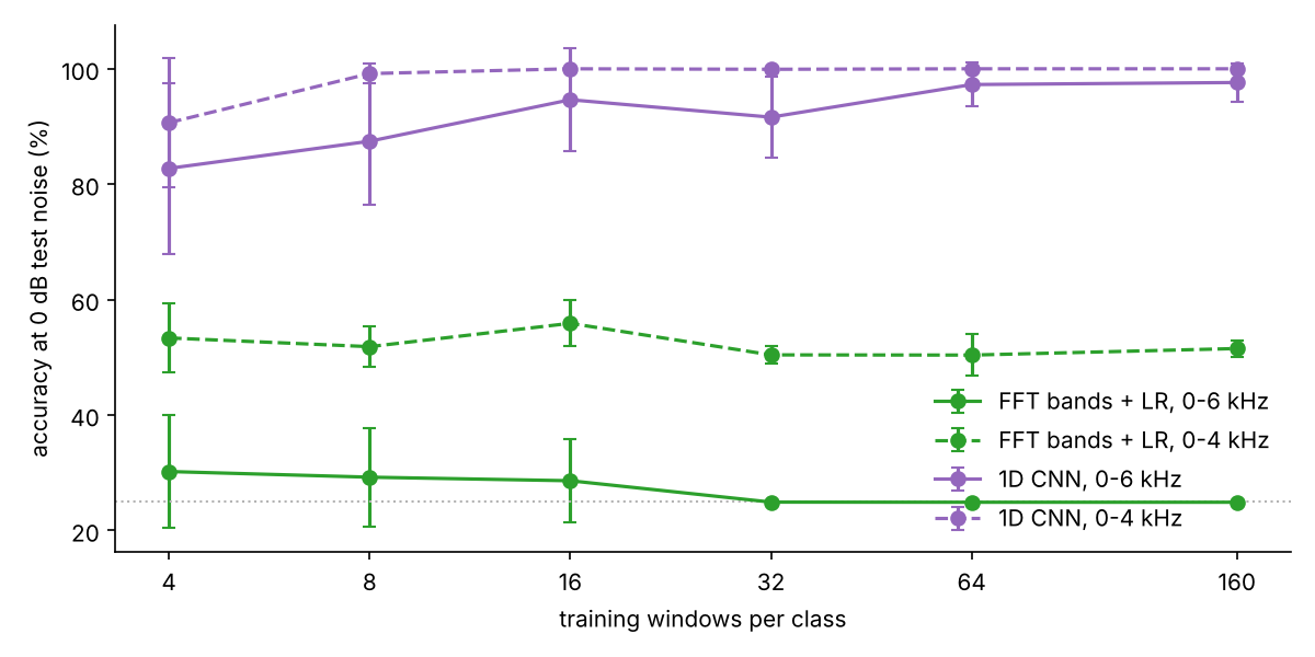
At 0 dB noise, the band-limited CNN already reaches 99.2% with 8 windows per class, and 100% from 16. With only 4, it averages 90.7%, but varies a lot from one random draw to another (±11 points).
The FFT model stays near 50–56% whatever the training size. More data does not help, because its problem is not too few examples. Its 64 averaged bands simply do not keep the information that survives the noise.
The CNN's advantage is in time. A fault is a train of short impacts, and a convolution filter that matches one impact still finds it under heavy noise; this is the same idea as a matched filter. Averaging the spectrum into wide bands throws that timing away.
What this experiment does not show
- The FFT model here is a simple one. The classic engineering method is envelope analysis: band-pass around a structural resonance, take the envelope, and look for peaks at the bearing's characteristic fault frequencies. It is built to handle noise, and it would likely do much better than 64 averaged bands. This comparison is "generic spectrum features vs a CNN", not "the best signal processing vs a CNN".
- Neither model saw noise in training. Training with noise added (augmentation) is the obvious next step, and would likely help the FFT model the most.
- One dataset, one fault size, artificial faults. Real faults grow gradually, and a real plant has other machines, speed changes, and sensors mounted differently. CWRU says little about any of that.
- Synthetic noise. White Gaussian noise is the easiest kind. Real plant noise has structure, often in the same bands as the faults.
Takeaways
- CWRU is too easy to rank methods on clean data. Both methods hit 100% with 4 examples per class. Test under noise, or on a harder dataset.
- Look at the spectra before training anything. The FFT model learned a difference in recording equipment, not in bearings, and only noise exposed it. A random train/test split would never have caught it.
- Against noise, the CNN won clearly, keeping 100% at 0 dB where the generic FFT model managed 51.5%, while needing only 8–16 labelled windows per class.
Run it yourself
git clone https://github.com/Ahmad-Nayfeh/portfolio-website
cd portfolio-website/notebook-code/bearing-fft-vs-cnn
pip install numpy scipy scikit-learn torch matplotlib
python experiment.py      # downloads 16 CWRU files (~70 MB) on the first run
Sources
- Case Western Reserve University Bearing Data Center: engineering.case.edu/bearingdatacenter.
- W. A. Smith and R. B. Randall, "Rolling element bearing diagnostics using the Case Western Reserve University data: A benchmark study," Mechanical Systems and Signal Processing, 64–65, 2015: a careful analysis of the dataset and of envelope-based diagnosis.
- W. Zhang et al., "A new deep learning model for fault diagnosis with good anti-noise and domain adaptation ability on raw vibration signals," Sensors, 17(2), 2017: the wide-first-kernel CNN (WDCNN) design used here.