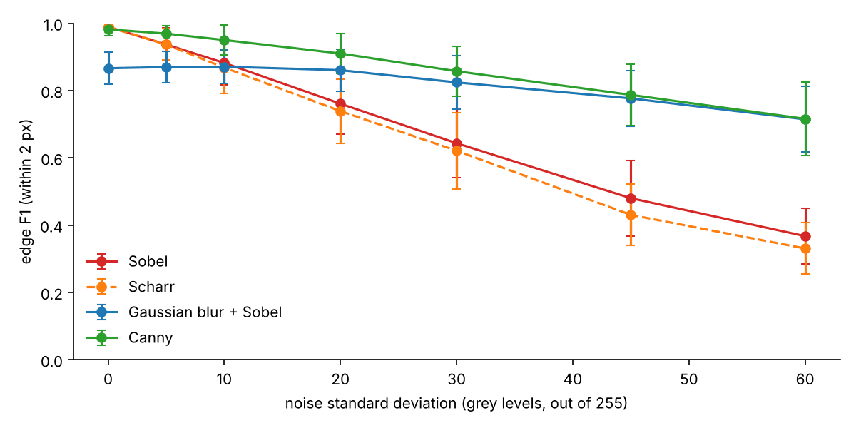
Edge detection is usually the first thing taught in image processing, and usually judged by eye: run three operators on a photo, put the results side by side, decide which looks best. That is hard to argue with, and hard to learn from.
This article measures instead. It asks:
- Does Scharr, the "more accurate" version of Sobel, actually detect edges better?
- How fast does each detector break down as the image gets noisier?
- What does Canny add on top of a plain gradient, and does it matter?
The code is in notebook-code/edge-detectors-noise. It runs in about 25 seconds and produces every number and figure here.
Measuring edges needs a ground truth
To score an edge detector you need to know where the true edges are. In a photograph nobody knows exactly, so I generate the images:
- Scenes: 256×256 pixels, with eight random filled shapes (circles, rectangles, triangles) at random grey levels, on a smooth gradient background.
- Real-looking edges: each scene is drawn at four times the size and then shrunk, so the edges are soft over a pixel, like in a real photo.
- True edges: wherever two regions meet. The gradient background has no edges, so a detector that fires on it is wrong.
Noise: Gaussian noise with a standard deviation of 0 to 60 grey levels, on a 0–255 scale. At 60 the image is very noisy, though the shapes are still clear to the eye.
The score: F1, which combines two questions.
- Precision: of the pixels the detector marked, how many are within 2 pixels of a true edge?
- Recall: of the true edge pixels, how many have a detection within 2 pixels?
F1 is their harmonic mean: 1.0 is perfect, and it drops if either one drops. Allowing 2 pixels of tolerance means a detector is not punished for being off by one pixel.
The threshold: every detector needs one (how strong a gradient counts as an edge), and the result depends heavily on it. To give each detector its best chance, the threshold is tuned separately for every detector and every noise level, on 10 scenes. Then it is scored on 30 other scenes.
The four detectors
- Sobel: estimates the horizontal and vertical derivatives with two 3×3 kernels, takes the gradient magnitude , and keeps the pixels above the threshold.
- Scharr: the same idea, with weights (3, 10, 3) instead of Sobel's (1, 2, 1). It is designed to be more accurate about the direction of the gradient.
- Gaussian blur + Sobel: smooth the image first (Gaussian, σ = 1.5 px), then Sobel.
- Canny: the same smoothing, then the gradient, then two extra steps. Non-maximum suppression keeps only the pixel at the peak of each edge, so edges are one pixel wide. Hysteresis keeps weak edge pixels only when they connect to strong ones.
def grad_mag(img, op, blur):
    x = cv2.GaussianBlur(img, (0, 0), blur) if blur else img
    if op == "sobel":
        gx, gy = cv2.Sobel(x, cv2.CV_32F, 1, 0, ksize=3), cv2.Sobel(x, cv2.CV_32F, 0, 1, ksize=3)
    else:
        gx, gy = cv2.Scharr(x, cv2.CV_32F, 1, 0), cv2.Scharr(x, cv2.CV_32F, 0, 1)
    m = np.hypot(gx, gy)
    return m / m.max()

canny = cv2.Canny(cv2.GaussianBlur(img, (0, 0), 1.5).astype(np.uint8), 255 * t / 2, 255 * t, L2gradient=True)
Results
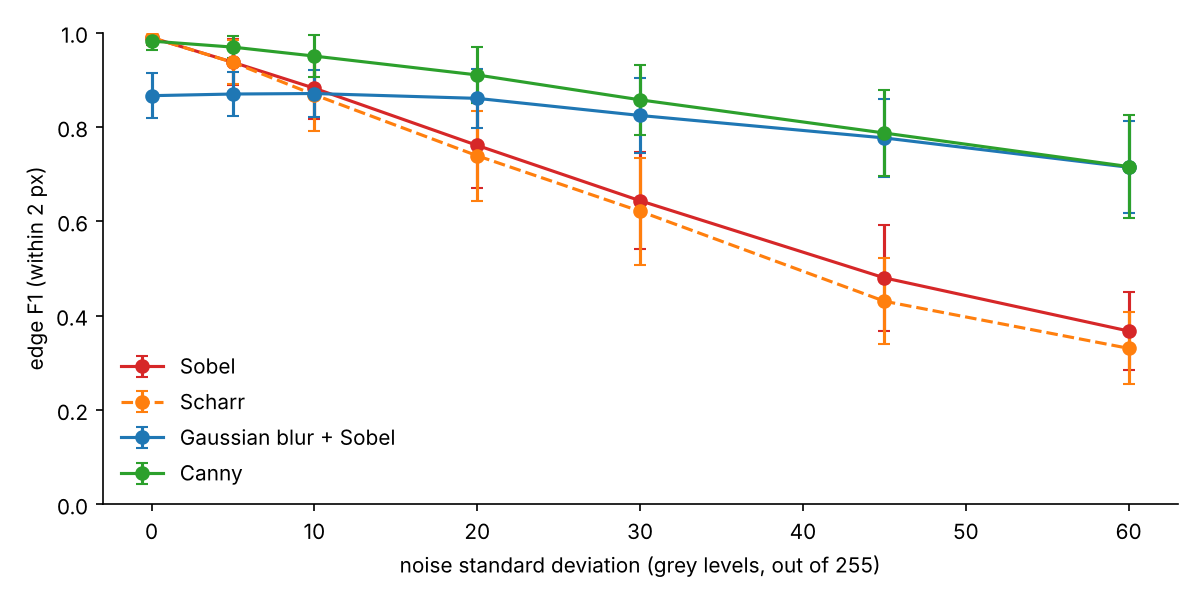
| Noise (sd) | Sobel | Scharr | Blur + Sobel | Canny |
|---|---|---|---|---|
| 0 | 0.989 | 0.990 | 0.866 | 0.982 |
| 10 | 0.882 | 0.868 | 0.871 | 0.950 |
| 20 | 0.761 | 0.739 | 0.861 | 0.910 |
| 30 | 0.643 | 0.621 | 0.824 | 0.857 |
| 45 | 0.480 | 0.430 | 0.777 | 0.787 |
| 60 | 0.367 | 0.330 | 0.714 | 0.716 |
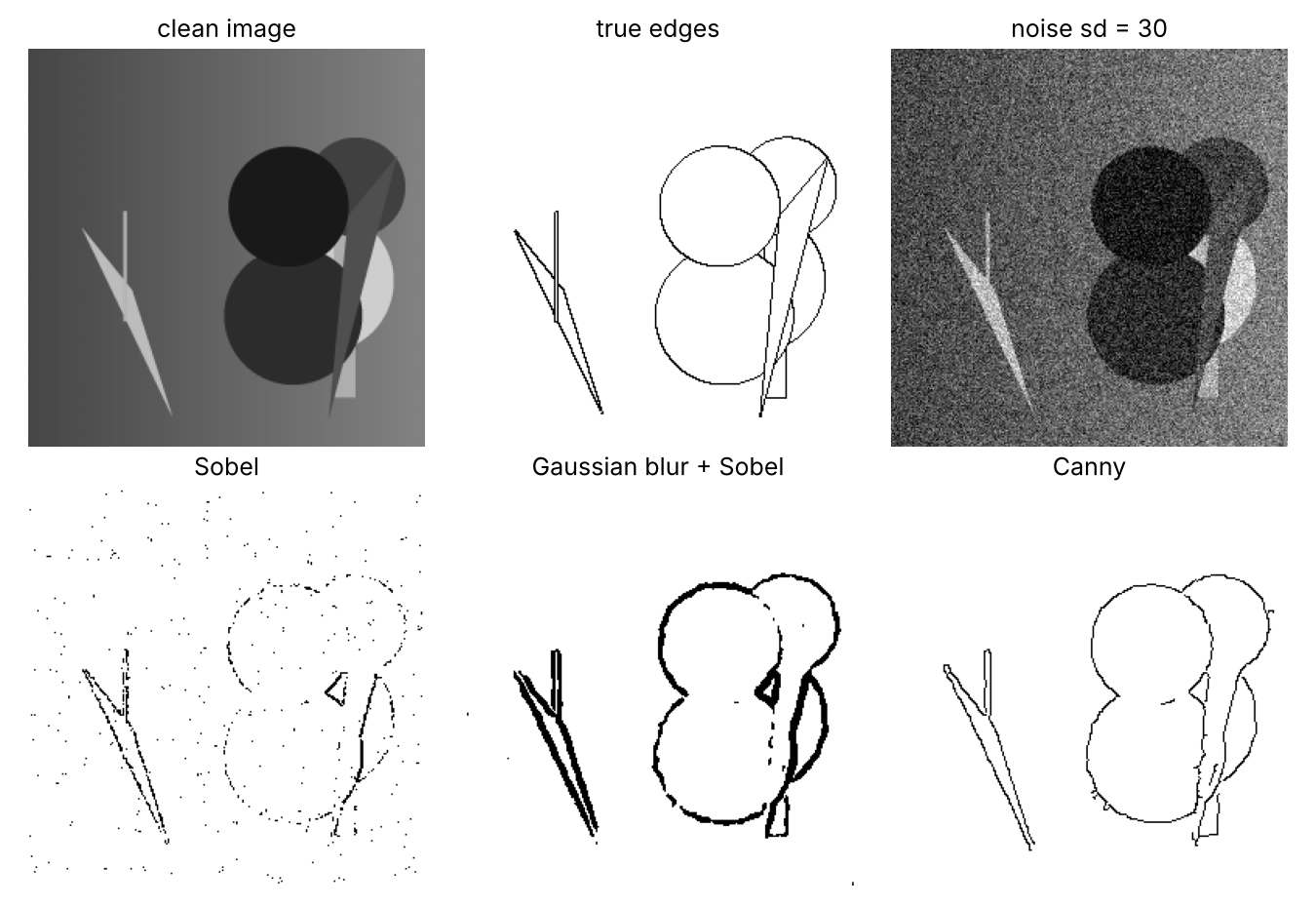
And what the detectors produce at noise 30:
What the numbers say
1. Sobel and Scharr are practically the same detector. On a clean scene their gradient magnitudes have a correlation of 0.9992. Under noise Scharr is slightly worse (0.621 vs 0.643 at noise 30), probably because its heavier center weight averages less across the kernel. Scharr's advantage is the accuracy of the gradient's direction, and an edge map does not use direction.
2. Without smoothing, noise wins quickly. Plain Sobel loses a third of its F1 by noise 30. Look at the "Sobel" panel above: noise pixels light up all over the background (precision drops from 1.00 to 0.78), while weak true edges sink below the threshold (recall drops to 0.58).
3. Smoothing trades sharpness for robustness. A Gaussian blur before Sobel nearly flattens the curve: 0.871 at noise 10, still 0.714 at noise 60. But on the clean image it is the worst of the four (0.866), because the blur spreads every edge over several pixels. The thresholded edges become thick bands, and the pixels at their outer sides are more than 2 px from the true edge. Its precision on clean images is only 0.85.
4. Canny is the two fixes together. Its smoothing gives the robustness of blur + Sobel; non-maximum suppression gives back thin edges, and with them the precision. It is the best or tied at every noise level from 10 up. At very high noise (60), Canny and blur + Sobel are equal (0.716 vs 0.714): both are limited by the same blur, and the thinning cannot recover edges that the noise has already erased.
The lesson is not "use Canny" so much as "the operator matters less than what you do around it." The choice between two 3×3 derivative kernels changed F1 by at most 0.05. Smoothing before, and thinning after, changed it by up to 0.35.
What this experiment does not show
- Synthetic scenes. Real photos have texture, shading and blur, and their "true" edges are a matter of opinion. On a benchmark of human-drawn edges, such as BSDS500, all four detectors would score far lower, and learned detectors far higher.
- One smoothing level. σ = 1.5 px for both blur + Sobel and Canny. Increasing σ with the noise level would help both at high noise and hurt both on clean images.
- Thresholds tuned per noise level. In practice you usually don't know the noise level in advance, so a real system would do worse than these curves unless it estimates the noise first.
- Only Gaussian noise. Salt-and-pepper noise, for example, calls for a median filter rather than a Gaussian blur.
Run it yourself
git clone https://github.com/Ahmad-Nayfeh/portfolio-website
cd portfolio-website/notebook-code/edge-detectors-noise
pip install numpy opencv-python-headless matplotlib
python experiment.py
Sources
- J. Canny, "A computational approach to edge detection," IEEE Transactions on Pattern Analysis and Machine Intelligence, PAMI-8(6), 1986.
- H. Scharr, Optimale Operatoren in der digitalen Bildverarbeitung, PhD thesis, University of Heidelberg, 2000: the derivation of the Scharr kernels for accurate gradient direction.
- R. C. Gonzalez and R. E. Woods, Digital Image Processing, 4th ed., Pearson, 2018: chapter on edge detection, for Sobel and the effect of smoothing.
- D. Martin, C. Fowlkes, J. Malik, "Learning to detect natural image boundaries using local brightness, color, and texture cues," IEEE TPAMI, 26(5), 2004: the precision/recall evaluation with a distance tolerance used here, in simplified form.